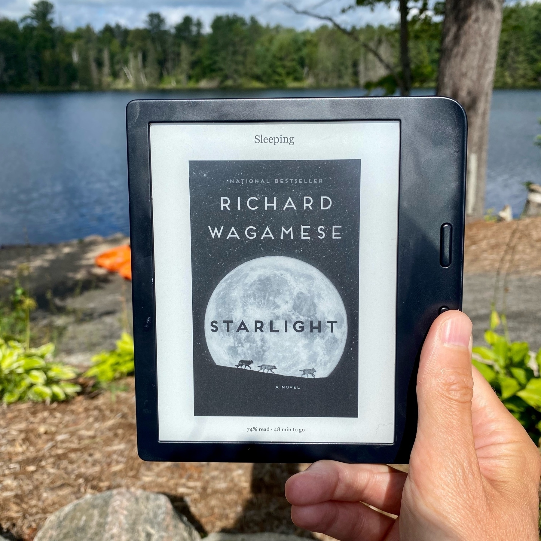
As a follow up to my earlier post, now that I’m on the eleventh book of my vacation, I can confirm that the Kobo Libra 2 is exactly what I’d hoped.
The screen has been easy to read in all lighting (especially bright sunlight on the dock), the page turn buttons are reliable, and the public library integration has been seamless.
After a few days of recovery, and before I forget, here are a few notes on the Tremblant 70.3 Ironman.
The short version (given there’s lots of details below) is that the course was fantastic and the race was really well organized.
Pre-race
This part was easy and the day prior to the race. There were scheduled times for registration and all we needed was the QR code from our online payment. With that, they handed over a wristband, timing chip, all sorts of stickers with my bib number, swim cap, t-shirt, and a morning gear bag for transferring clothing from the swim start to the run finish.
Next up was dropping my bike off at the transition. There were two stickers for the bike, both of which had my bib number on them and matched the number on my wristband. Staff at the transition entrance used these to make sure the bike belonged to me, before letting me in. Then I tracked down my transition spot, which was at the bike start end of the transition zone.
They also had a mandatory athlete’s briefing in the afternoon. As a first timer, this was really helpful. They talked through the overall course, showed some specific turn arounds and tricky spots, and then reminded us of the important rules. There were also repeated (and welcome) warnings that race day was going to be exceedingly hot (at least for recently hibernating Canadians) and that everyone needed to take precautions.
That was it for the Saturday events, other than finding some food and trying to get a good night’s sleep. Sunday (race day) started early, so that I could get the rest of my transition spot set up by 6:30. As with the bike, they checked wristbands before letting anyone in. I took about 10 minutes to get everything organized and visualize how I’d move through the zone.
Swim
Although the novelty might wear off after a few more races, standing on a beach with 2,000 other people along with a strong mix of excitement and anxiety is quite the experience. People were in and out of the lake to get in a warmup swim before the start and then the national anthem played just before 7. The pro men started right at 7, followed by the pro women at 7:05, and then the rest of us started at 7:10. We were all self organized into corrals of different expected finish times and I aimed for the back end of the 34-37 minute corral.
Rather than one big mass start, there was a gate system at the start of the swim that let six swimmers through every 10 seconds. This kept a steady stream of swimmers going through the start without a giant crowd. The only downside was that it took a while to clear the beach. The pro men had already started their bike rides before I’d even left the beach! I crossed the start line at 7:32.
Not much to say about the swim. The water was a nice, cool temperature and there were only a few spots around the half-way point where there was any significant contact with other swimmers. This was mostly because at that point we were swimming directly into the sun and seeing the buoys was really challenging. We all just kept swimming forward, assuming that anyone in front of us was headed in roughly the right direction and it all worked out.
I saw at least three people getting hauled out of the water by the safety teams that were paddling around in canoes and kayaks. I can only imagine how difficult it would be to need to quit the race so early, but safety is so much more important than pushing through and risking serious injury.
One challenge I had with the Milton sprint triathlon was significant dizziness at the end of the swim and, consequently, a challenge getting through T1 on the bike. So, this time I slowed down near the end of the swim and tried to more carefully move from vertical to horizontal while getting out of the water. This seemed to help; although I still felt a bit light-headed, it wasn’t nearly as bad as last time.
33 minutes for the swim was faster than I’d planned, though I felt good throughout. So, I wasn’t worried.
The swim ended with a 200m run into the transition zone. During this, I was able to wiggle out of the top half of my wetsuit, in preparation for the rest of the transition. Once I was at my transition spot, I pulled off the wetsuit and quickly consumed one caffeinated gel. Then helmet on (they’re really strict about not touching your bike without a helmet on), bike shoes on, and grabbed the bike to run out to the bike mount line.
Bike
The bike course was gorgeous. Lots of hills through Canadian Shield and forests on (mostly) smooth asphalt. There was a really steep downhill around km 16 that got me up to about 79 km/h and, since this was part of a loop, I also had to climb back up this hill on the way back. I’d been worried about this when looking at the map. But, in the end, it wasn’t so bad. I knew it was coming and just had to power through. The part that surprised me was the undulating hills in the last third. Despite the great scenery, these were really hard!
My coach had advised I keep my heart rate around 155 throughout the bike course. Other than a few of the climbs, I was able to stick to this. It was actually really helpful to have a specific target to keep trying to hit. Three hours on the bike can get rather tedious without something to focus on and there’s always a worry about pushing too hard on the bike and blowing up on the run.
There were four aid stations on the bike course. Given the heat warning, at each one I grabbed a 750mL bottle of water. 2/3rds of the water I sprayed onto my head for cooling, the rest I drank. They had kids at the end of each aid station with hockey nets and sticks. You threw the empty bottle towards the net and they stick handled them in for disposal.
I also had a 750mL bottle of electrolytes and 500mL bottle of water on the bike that I consumed throughout, along with two Stroopwafels and two energy gels.
2 hours and 56 minutes on the bike was a few minutes faster than I’d anticipated. So, also happy with this. By the end of the 90km, my legs felt reasonably fresh, but I was glad to get off the bike. Things were starting to get pretty uncomfortable. This might partly have been because it was actually my first ever ride with aero bars. I wouldn’t recommend waiting until a race to try these out, though that was how it worked out for me. Overall, I’d say the aero bars were more comfortable than I’d expected, I just wasn’t used to them.
Run
T2 was straightforward. I racked my bike, took off my helmet, and switched to running shoes and a hat. One more caffeinated gel and off I went.
My plan was to maintain a 5:30 minutes/km pace for the run with an emphasis on keeping it slow after the bike transition (it is really tempting to start running fast off the bike). This was sustainable for about the first half. By the second half, though, the heat really started catching up with me and I had to slow down to around 6 minutes/km. I was super sensitive about pushing too hard in the heat and, consequently, jeopardizing actually finishing the race. So, I wasn’t upset about slowing down. I did see at least two people off to the side of the course being attended by medics with apparent heat stroke, which were good reminders to pace carefully.
I’d committed to myself before the race that I would walk through each of the 12 aid stations. At each one, one water went onto my head, another I drank, and then I grabbed a couple of cups of ice. I had a small ziplock bag that I put ice in to hold, while the other ice went down the front of the Triathlon suit. Like me, many of the runners were making lots of jiggling noises as the ice that had fallen down into our shorts bounced around. Absolutely necessary though, given the heat and humidity.
For nutrition on the run, I had two gels: one at about the 10km mark and the other around 15 km.
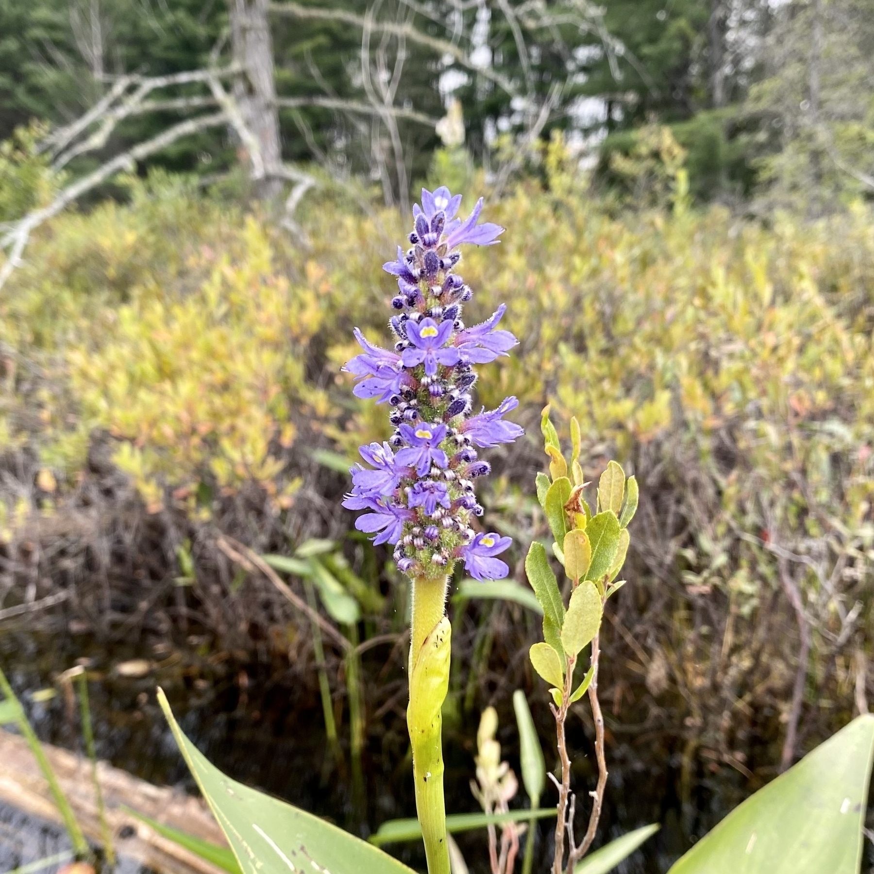
The run course was also gorgeous. We ran through a decommissioned rail road track converted to a multi-use recreational path through the heart of the Laurentians that included waterfalls and forested areas. Although not as shaded as I’d hoped, the course was great. There were also a few spots with sprinklers or fire hydrants spraying water. These were helpful for cooling down. I was particularly amused by the local resident that was lounging in a lawn chair with a beer in one hand and hose in the other. A bit of eye contact and thumbs up was all you needed to have him hose you down on the way by: so refreshing!
Kilometres 14 to 17 were pretty tough. I was far enough along to be pretty tired, but not yet quite far enough to know that it was almost over. Knowing my family was at the end, ready to cheer me on really helped here.
The last km of the run was an extra experience. You run right down the hill through the middle of the Tremblant village with spectators cheering you on from either side. Despite all the hard work up to this point, you really feel pretty energized for this part, especially when you finally see the finish line up ahead.
2 hours and 3 minutes for the run was just a few minutes slower than I’d anticipated. I was totally happy with this time, given everything that preceded it and the heat.
Post-race
The finish line funnels you into a big tent with picnic benches. There were plenty of cold drinks available, along with a plate filled with pasta and french fries. I grabbed a couple of waters and then made my way out of the tent to see my family. I was pretty focused on that point with seeing them and then getting into the lake to cool down.
My main goal had been to finish the race. That was accomplished. My second goal was to be in the top half of finishers. I managed to be in the top 1/3 for my age group and top 1/2 overall. So, I was very happy with my overall results.
I felt that I executed the race well. No issues with hydration or nutrition, along with an intentionally conservative level of effort to maximize my chances of finishing the race worked out well.
Two minor lessons learned: more sunscreen, I burned the back of my shoulders pretty thoroughly; and some more lubrication under the zipper of the Triathlon suit, I still have a pretty good friction burn in the middle of my chest.
All things considered, my symptoms aren’t too bad, which I’m grateful for. Nonetheless, I’ve mostly been in bed for a couple of days to properly recover.
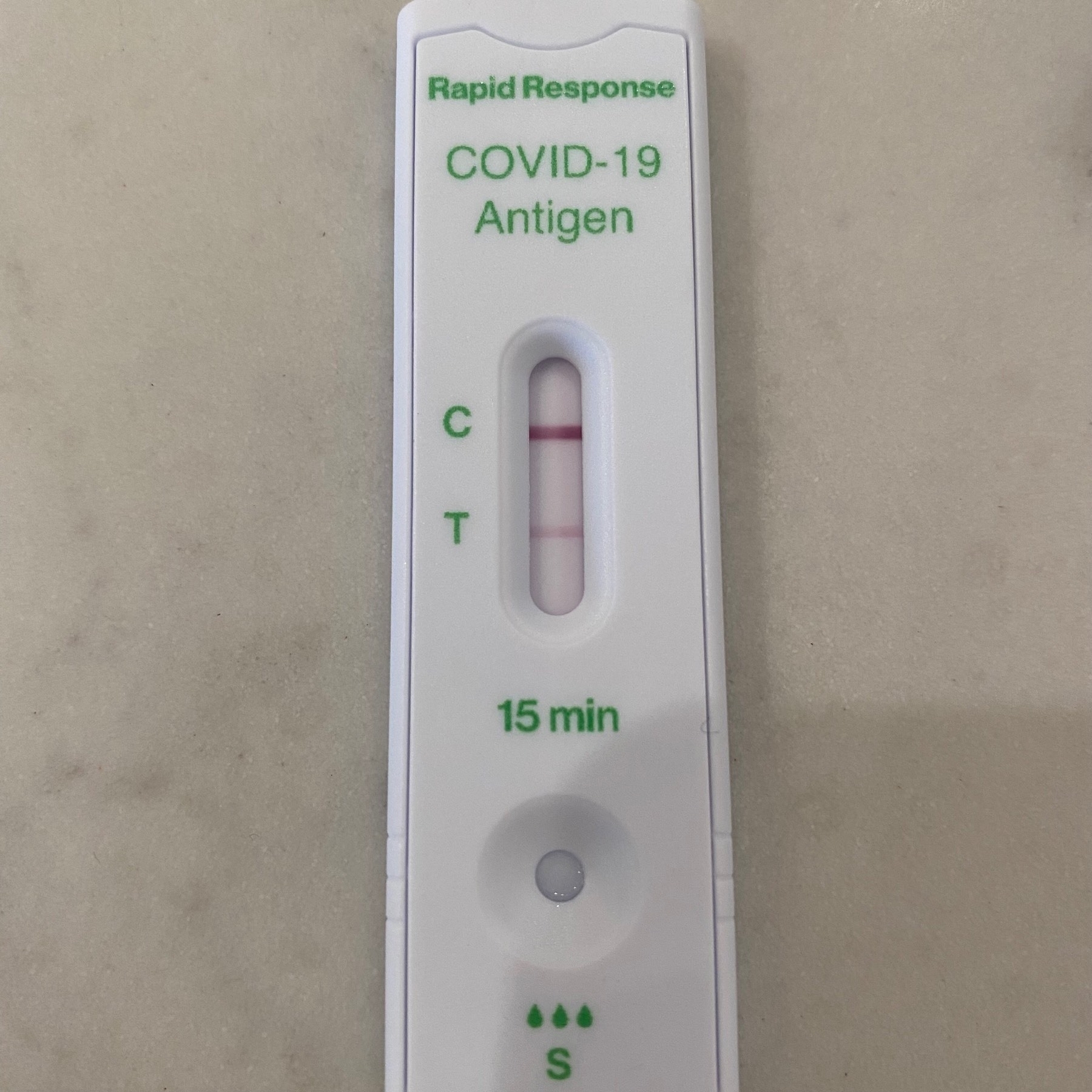
Since I’ve been monitoring my Readiness To Train (RTT) score, I was curious to see how COVID would appear in the metrics.
Thursday morning was the first indication that something was wrong. I completed what felt like a reasonably strong swim workout, only to suddenly feel really drained of energy while walking home from the pool.
After dragging myself home, we found out my son’s friend had tested positive. So, both he and I took a rapid test that confirmed we were infected.
Thursday night was peak symptoms for me, producing an abysmal RTT.
All morning in bed on Friday helped a lot and then a much better sleep last night layered improvement on top.
Today’s RTT seems rather optimistic to me though. My planned intensity included a two hour bike ride and 20k run. Those are not happening! Today’s planned intensity will be watching the season finale of Severance in my pyjamas.
My experience with RTT is that it typically reinforces how I actually feel with, perhaps, the occasional early warning. Basically a second opinion that reinforces my intuition. But when we disagree, like now, I’m definitely following how I feel.
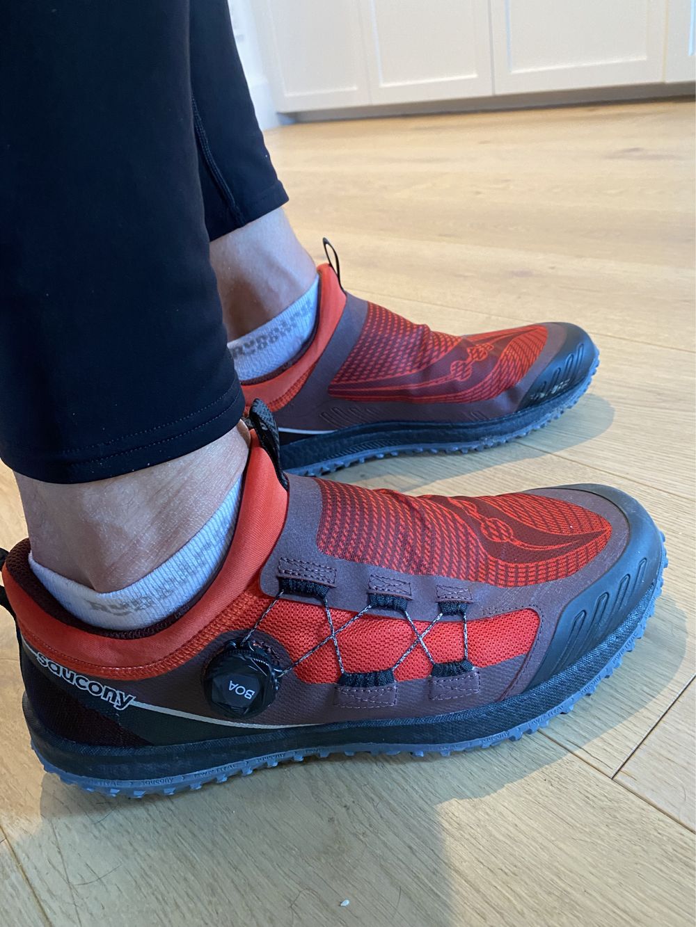
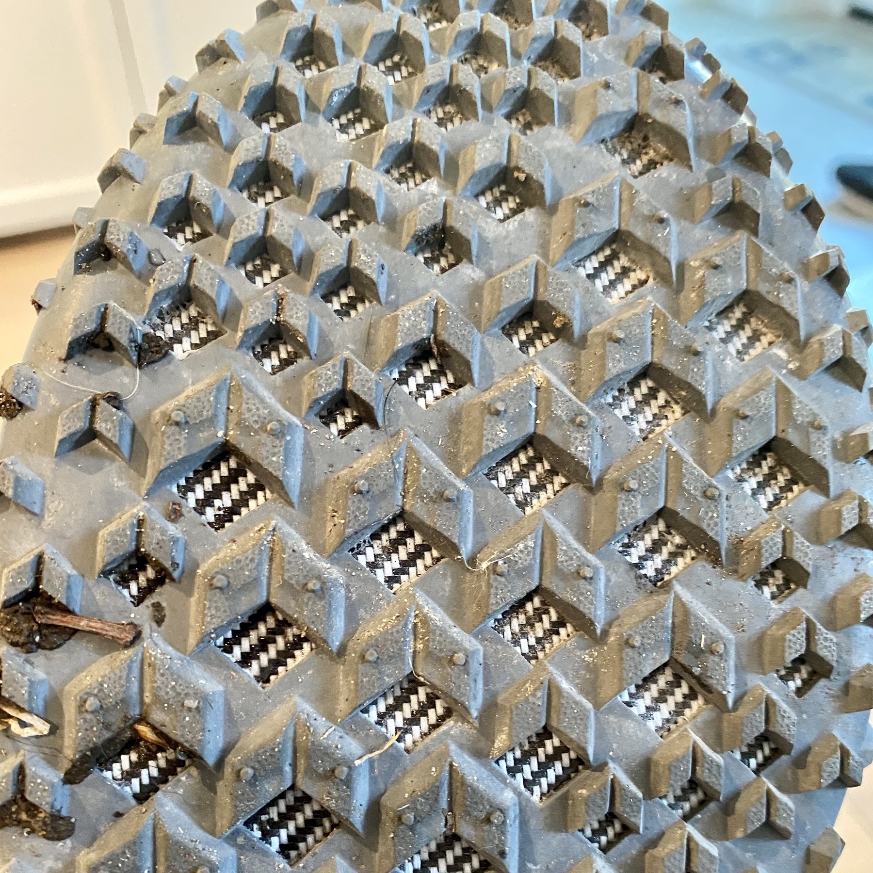
I added a new pair of running shoes to my closet: Saucony Switchback 2. They are a lightweight trail shoe with the BOA Fit System (rather than laces) and good treads for gripping.
I took them out for a 10k run around the neighbourhood. Not quite the right conditions, since I was mostly on sidewalks and they’re trail running shoes. Despite that, the shoes felt fast and light. For the first couple of kms, I felt a bit like I was slapping my feet on the ground, since I’m used to more cushioning and my feet weren’t making contact quite when I was expecting them to. I didn’t take long to adjust to a better form though. I’m curious to see what the transition back to my usual shoes is like. Presumably with practice, I’ll be able to switch back and forth easily.
Overall, I’m happy with the new shoes and look forward to getting out to an actual trail with them.
I’m still using MindNode for task management. Seeing all of my tasks, projects, and areas of focus on one mind map has been really helpful, especially since it is integrated with Reminders.
One challenge has been integration with Mail, given the majority of my tasks arrive via email. Despite Apple’s seemingly inexplicable decision to isolate Mail from the usual sharing actions found in other apps, they at least allow drag and drop from Mail into Reminders, which adds a link to the original email message. This works with MindNode too. If you drag an email onto a node, it will add a link there. The issue is that when you synchronize MindNode with Reminders, the links to emails from MindNode no longer work when shown in Reminders.
After tinkering around for a bit, there’s a relatively easy fix. When you drag a mail message to a node in MindNode, it adds a url that looks something like:
message:%3CYT2PR01MB9@YT2PR01MB9447.CANPRD01%3E
Editing the link to add // after message:makes the link work in Reminders, while also continuing to work in MindNode.
I’m not sure why MindNode creates a url that isn’t accessible from other apps (perhaps a security feature?). At least this fix, though a bit annoying, allows for a more seamless integration between Mail, MindNode, and Reminders.
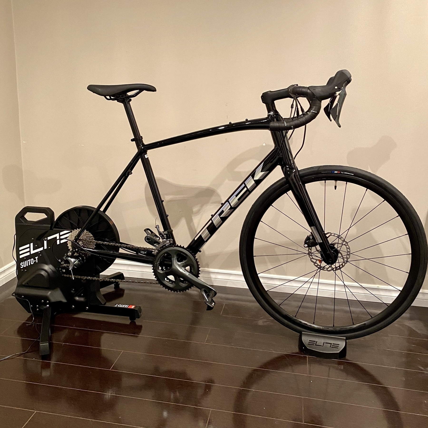
The last piece of my training setup was an indoor bike trainer. Canadian winters aren’t great for outdoor cycling (-20ºC with a blizzard just a few days ago, for example). So, I picked up an Elite Suito-t which is well reviewed and on sale at my local bike shop. This is a direct transmission model with built in power and cadence sensors.
I don’t have enough space in my house for a spot fully dedicated to cycling. So, I’ve got the bike a trainer tucked in a corner of the basement and then I slide our basement couch out of the way and move the bike in front of the TV when I’m riding. The compact size of the Suito definitely helps here.
The Suito came with a free month of Zwift that I’ve really been enjoying. Zwift has lots of group rides and workouts that are fun (though hard work!). Because the Suito is a smart trainer, it automatically adjusts resistance to mimic hills, as well as hit specific targets during structured workouts. Riding with a hundred or so people from around the world is inspiring and motivating.
Although I’m really looking forward to proper outdoor rides in the spring, this indoor setup has been great.
I knew going in that a first triathlon requires a lot of planning and gear, especially when you don’t have any equipment.
Given that the cycling component is the longest distance, it is important to have a good bike. Once I knew my size, the next step was to actually choose a bike. And, oh my, are there decisions to make.
As with most things, budget sets a pretty useful constraint. Within that, there’s finding the sweet spot between spending enough to get something good that you won’t regret compromising on later and spending so much that you’ve exceeded your fitness level and can’t capitalize any speed gains from the purchase.
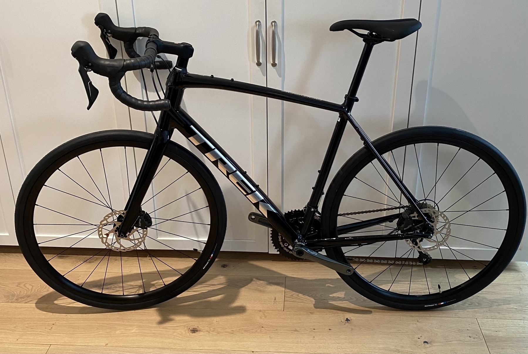
My bike sizing was based on a Trek Domane and I figured that was a good place to start. The next choice to make was between aluminum and carbon fibre. The obvious difference here is price. This Global Cycling Network video helped me understand that an aluminum frame is more than sufficient for me. Spending a few thousand extra dollars to gain a few minutes advantage in a “fun” race is a bad choice. Consistent training is going to provide a much better advantage than the choice of bike frame.
Having made it this far, I figured it was time to start looking around for options, only to find out that COVID had disrupted yet another supply chain. There are close to zero new or used bikes in the market. In fact, there was exactly oneTrek Domane AL 4 in Toronto with the next nearest one 200 km west in London. The AL 4 seemed like the right balance of cost and performance for me. So, that’s now my bike!
After all that, I now have the fanciest bike (by far) that I’ve ever owned and it is -20ºC outside just after the biggest snow storm in decades. Rather than just stare forlornly at the bike for the next few months, my next purchase will be an indoor trainer, so that I can build up cycling fitness while winter carries on.
I’ll be spending many hours and a reasonable amount of money on a bicycle over the next few months. To be efficient, comfortable, and injury free, I want the bike to fit me closely. So, I sought the advice of Scott, a professional bike fitter.
Scott has an interesting contraption that is the various parts of a bike, each adjustable, with which he can recreate any frame geometry. He started out with a Trek Domane as a reference point and had me ride it for a few minutes. Then with an assortment of rulers, protractors, and lasers, he measured me, moved parts, measured again, and optimized the fit. Once the fit was established, he generated a detailed report for me of all the various lengths and angles that I can use to confirm the size of any bike that I find.
I also learned that my tibias are longer than my femurs (not by much) which is not typical (most people have longer femurs). This ends up affecting my optimal bike geometry, since it affects the angle of my knee and hip when at the top of a pedal stroke.
Now that I know what size of bike to get, I’m on the search. The COVID-induced supply chain challenges are definitely affecting availability.
As an experiment, I spent the past week listening only to the Activity Playlists in Apple Music. So, whatever I was doing, I picked the most closely related playlist.
Often these were straightforward. Cooking dinner with help from the kids: Cooking with Family; triaging the morning inbox of email: Checking Email; mind mapping a project: Brainstorming.
Other times it was more mood oriented. Reading by the fire when it is -20ºC: Winter; augmenting an early Wednesday morning coffee: Wake Me Up!.
Overall, the playlists are good.
The ones I listened to are meaningfully distinct from each other and the song choices do match the general mood of the activity. Just as one example, although their names are quite close, I did get different vibes from the Deep Focus, Peaceful Focus, and Creative Focus playlists.
In general the song choices are, not surprisingly, oriented towards the pop genres. That said, they aren’t just a collection of current hits. Playlists include some old gems and more obscure songs. Clearly, the songs were chosen with care and not strictly driven by machine learning algorithms.
One unanticipated side effect of this was that the rest of the family noted how much better the music was in the kitchen. No more of that “weird Dad music” 🙄. I take some consolation in the knowledge that in about ten years they’ll rediscover and appreciate these “classic songs” and finally realize that, in fact, I do have good musical tastes.
Although the music is generally good, discoverability is terrible. MacStories pointed this out and created a very helpful Shortcut for grouping and playing these playlists. Even when you select “See All” from the Just Ask Siri section, Apple Music shows some random selection of the playlists. I haven’t noticed any particular pattern of which ones are displayed and can’t understand why Apple is making it so difficult to browse them. Maybe they’re still experimenting?
I never did find reasons to listen to many of the playlists, like the whole series for Zodiac signs or the one for square dancing. This just shows the diversity of playlists available and, again, points out the problem with discoverability.
This was a successful experiment that forced me to actually experience the feature. That said, I wouldn’t want to continue relying on only these playlists. I’ll keep using them when I can’t be bothered to carefully choose an album or playlist and just want something appropriate to the mood or activity, which surely is the whole point of them anyway.
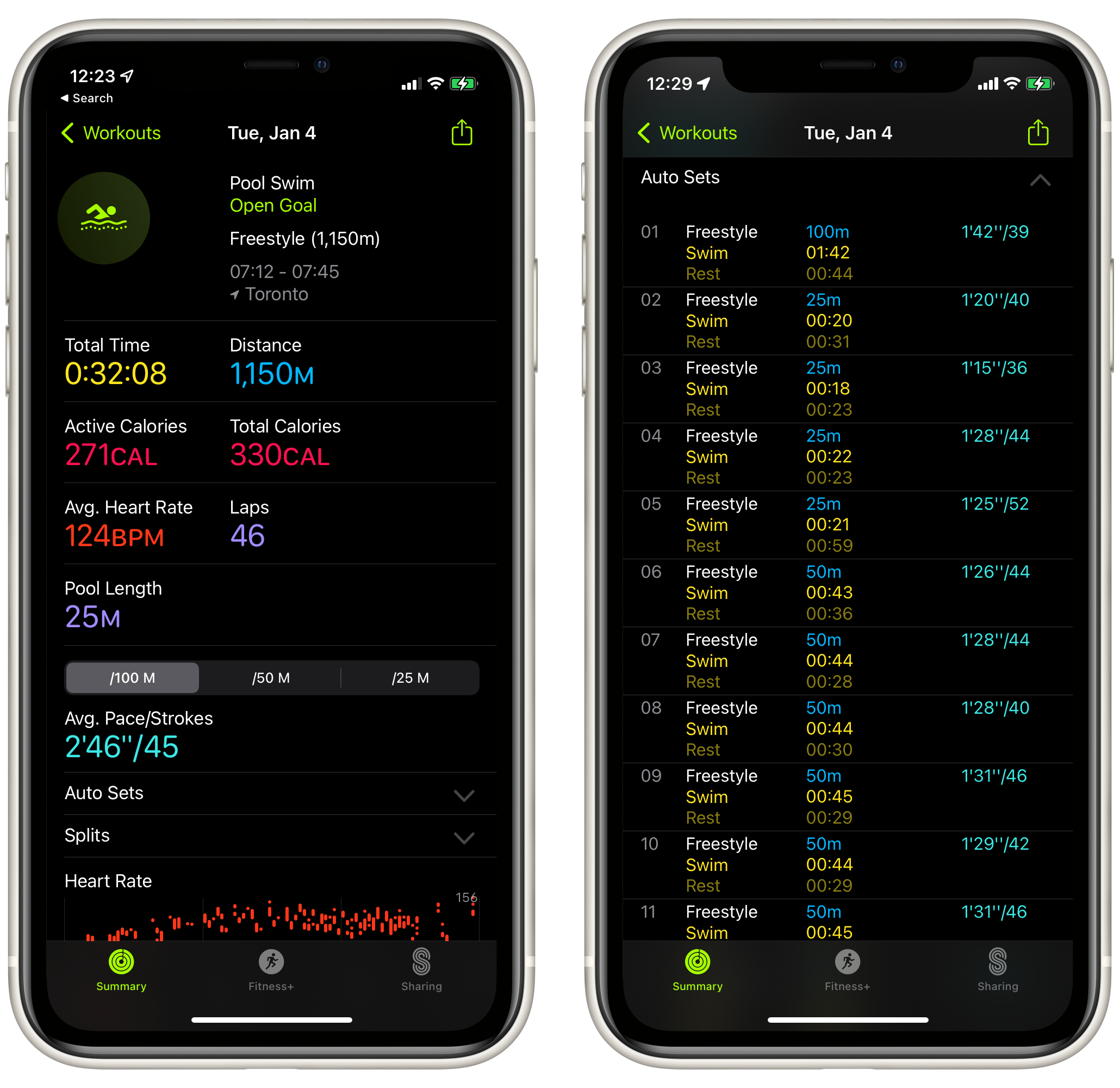
I’ve been in a pool with my Apple Watch before, though only either to splash around with the kids or with a beer at an all-inclusive resort. Today was the first time I’ve used it for an actual swimming workout. It has also been a long time since my high school swimming days back in the early 90s. So, an important day!
My coach gave me a straightforward workout:
Warm up 2 x 50m and 4 x 25m
Main set 10 x 50m with 20s rest and 10 x 25m with 20s rest
2 x 100m with 1 min rest
As expected, using the Apple Watch was simple. When you start up the workout, it asks for the length of the pool and then automatically figures out when you stop for a rest. This shows up in the “Auto Sets” in the screenshot below. Based on this, it looks like my rests were longer than planned, though I’m not entirely sure how precise these are and when it decides to start and stop. Something to keep an eye on next time.
I enjoyed being in the pool again and my muscle memory seemed to return. Way back in high school, I specialized in the 1,500m and was very familiar with the seemingly endless flip turns of a pool swim. One thing I need to work on is breath control. I’ve gotten very used to just breathing whenever I want and had some trouble getting in three strokes before breathing near the end of the workout. No doubt this will improve with practice.
I also need to work on my wardrobe. I was the only one in the pool wearing board shorts and no swim cap 😀
Through 2020, I built up an ornate system for tracking my time for both work and personal projects (like this one for reading). For most of 2021, I found this tracking really helpful.
I need to track my hours at work anyway, so using Timery and Shortcuts to automate much of this has been great. Having a strong sense of how long things take and ensuring good balance across projects are all benefits of time tracking.
For personal projects, though, I’ve been starting to feel a bit stressed by having a timer always running whenever I’m doing something, almost like I’m always in a race. At first, knowing how much time I was spending on particular things was great for my Year of the Tangible intention. This is well established now, and I haven’t been using the time reports for any personal projects. So, why am I creating anxiety for no benefit?
I’ve turned off all of my time tracking automations for personal projects. Despite some annoying bugs, ScreenTime is a good-enough replacement for keeping an eye on time spent on things like YouTube and social networking. A nice side benefit is that this also reduces the number of Shortcuts and other automation that I need to manage, allowing me to just enjoy my personal time.
Of course, I’ll keep tracking work projects, since the benefits far outweigh the costs there.
When I ran a marathon several years ago, my training plan was just to go for countless long runs. Now that I’m older and wiser, I’m going to be more sophisticated in training for Tremblant and that means getting a good coach.
The first question any potential coach has asked is: what is my goal for the race? This is a helpful first sign, since their approach to my training really should be based on my goal. Plus, it has been a good motivator for me to actually share my goal out loud, which helps me think it through.
My goal is to simply finish, while enjoying the race. I’m not aiming for any podium. Although I know it will be tough — the challenge is part of the point, after all — I want to avoid crawling across the finish line, bruised and battered after a long grind. My broader purpose is to use the event as a good excuse to keep active and try out new things. I hope that I’ll be doing events like this for the next decade or so. If the training burns me out or causes injuries, in the pursuit of some unattainable ranking at the event, we’ve missed this purpose.
I’ve also been thinking through what I’m looking for in a coach. There are lots of potentially valid approaches to coaching. I need to find one that aligns with my needs and expectations. In general, there are three things, in order, that I’m looking for.
Knowledge: There’s so much to learn! As I said at the beginning, there’s the training plan that mixes all three sports in the right amounts without causing injury. There’s also sorting out nutrition for the race to keep energy optimized. And gear (so much gear!) from bikes to wetsuits and apps to goggles. Without good advice, I could waste a lot of money on shiny, unnecessary gadgets. A seasoned coach can help with all of this.
Community: I’m generally autonomous and would naturally orient towards doing much of my training solo. Despite this, I joined a running group about a month ago and have really enjoyed the camaraderie and support. So, I’ll be looking to a coach to help get me connected with the local community, especially for the cycling. Long-distance rides will be much better with other people.
Accountability: I think I’m pretty goal oriented and persistent (some would say stubborn). I don’t yet know if this will persist over 6 months with significantly more training. Having a coach track my progress, adjusting where necessary, will help keep me honest and on target.
Inspired by @cedevroe’s semi-regular purges, I’ve gone through my many services and unfollowed, unsubscribed, and deleted everything. And, I mean everything! That’s all of my RSS feeds, newsletters, podcasts, and Micro.blog, Twitter, Instagram, and YouTube accounts. This seemed kind of crazy at first, until I realized that being so attached to these things is rather silly.
Before simply resubscribing to everything, I’m trying to take a more thoughtful approach to why I’m using each of these services.
All of my news feeds are in NetNewsWire with Feedbin as the back end. I’d accumulated a few dozen feeds here, the vast majority of which I was consistently just marking all as read. Many were feeds that I thought I should read, rather than actually wanted to read. I’m going to resubscribe to just the ones that seemed to consistently yield interesting (to me) articles, like Quanta Magazine and Aeon.
As newsletters arrive, I’ll unsubscribe from them. If I still see value, I’ll transition them over to Feebin and they’ll show up among the news feeds. Conceptually this makes sense to me, since they really are just another source of news, rather than actual correspondence to me.
Although I cleaned up my podcasts a couple of years ago, I’d added a few more since then. I think my original list is still the right one. Nevertheless, I’ve unsubscribed from them all and will reintroduce them slowly.
Instagram used to be where I went to see pictures from friends about their adventures, kids, and pets. Over time my feed had become dominated by brands, especially fitness, beer, and whiskey. Nothing wrong with any of these, obviously, just not what I need to be seeing, So, back to just accounts for people I actually know. As an aside, I was surprised by how easy Instagram makes it to unfollow, including a helpful list of which accounts you interact with the most and the least.
I really like the idea of Twitter as a place to follow my interests. We all know that in practice it can be a pretty nasty place. As an experiment, I’m going to try only following topics there, rather than people. To be honest, though, I lost my Twitter scrolling habit about halfway through the Trump presidency and I’m not that tempted to return.
Micro.blog was tricky. As the opposite of Twitter, I’ve found lots of nice people having interesting conversations there on a wide array of topics. But, the point of this exercise is to clean out everything, so even here I’ve stopped following everyone. I suspect that I’ll end up mostly back where I started on this one.
I have to admit feeling a bit disoriented this morning. My usual routine is to scan through all of these sources while waking up with some coffee. There are lots of other things I can be doing in the morning though, starting with actually reading some of the articles I’ve accumulated in my ever lengthening read-it-later queue.
Although a purge like this can seem dramatic, I think it can also be therapeutic. Thanks to @cedevroe for prompting this.
In preparation for Tremblant, I had my gait analyzed to find out if there are any issues with my running form. I found the process surprisingly thorough and interesting.
Katie (a registered physiotherapist) started out with a general discussion about my running history and goals. Then she filmed me running on a treadmill for about five minutes. We set a fast pace, since that quickly exposes any sloppiness in my running. I have to admit that watching myself running in slow motion was a bit awkward, though my form wasn’t as bad as I’d imagined.
Katie identified two issues: too much side to side rotation of my arms and a pronounced dip on my left side.
The arms are pretty easy. I just need to be more mindful of how they’re swinging and focus on moving them forwards and backwards, rather than side to side. This better directs my energy towards forward movement.
The dip is more complicated. Katie tried a bunch of different strength tests to isolate the muscle and we found that my left glute was much stronger than my right, which is odd, given I’m right handed. To distinguish between strength and muscle activation, Katie tried an acupuncture needle in my right hip. Remarkably, just a couple of minutes later, I was then much stronger on the right side. We did another round on the treadmill and my hips were now nicely aligned.
This suggested to Katie that my strength is fine, rather it’s insufficient muscle activation that is leading to the dip. She prescribed some warmup exercises to help. I know that I have a deficient warm up routine (as in there isn’t one, I just start running), so this is a good excuse to improve this component of my running routine.
As someone that generally just puts on running shoes and gets going, I’m glad I put in some time to understand my gait and identify some opportunities for improvement. I hope to be running for many more years and this should help minimize injuries.
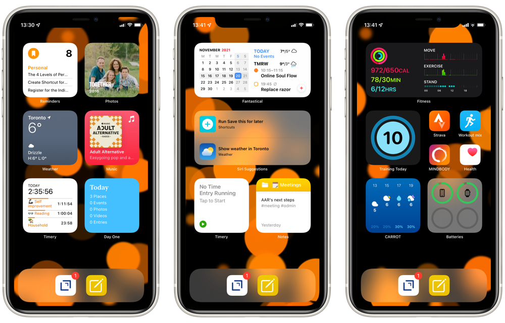
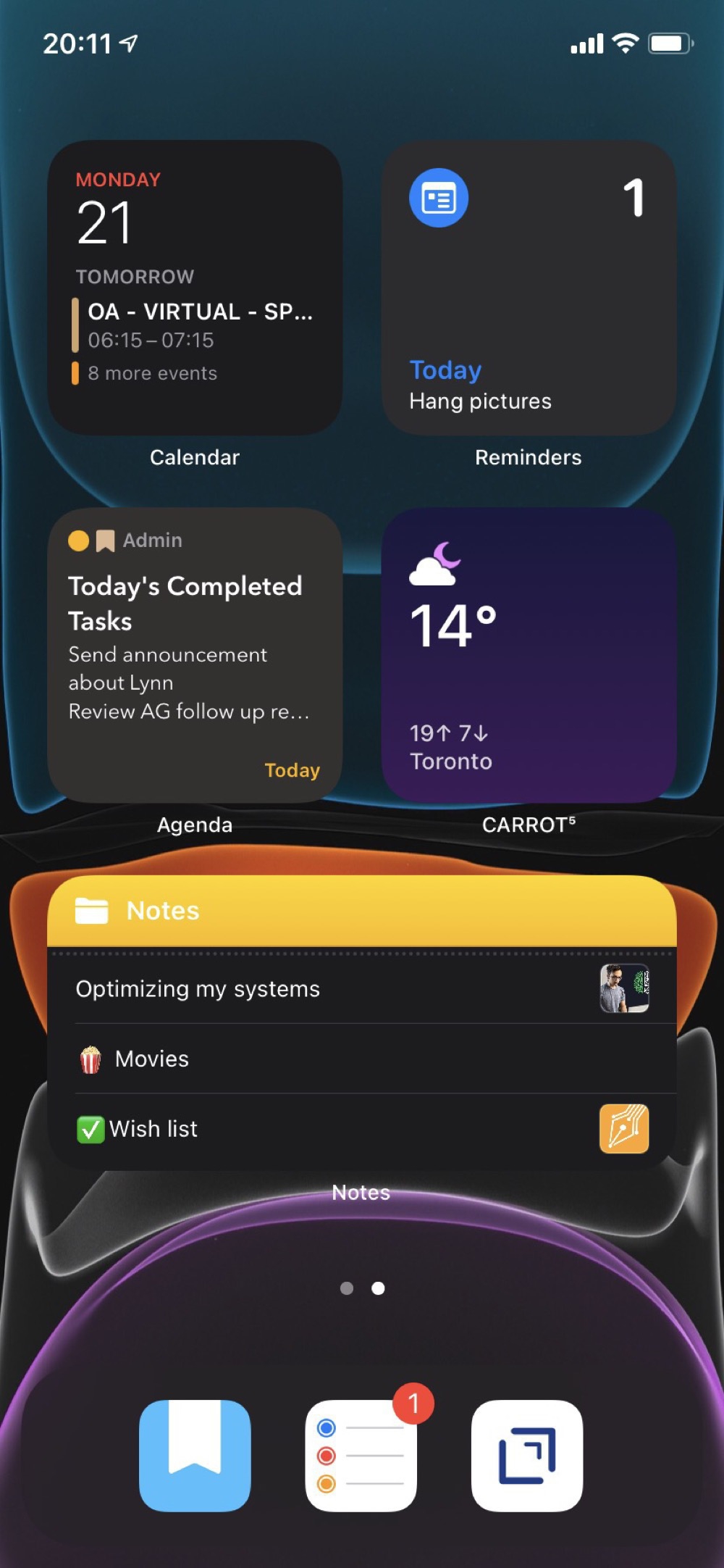
My iPhone Home Screen continues to evolve and, now that we have Focus Modes, I’ve made some further adjustments.
From left to right, I’m using three different Focus Modes: Personal, Work, and Fitness. The first two are entirely widget focused, while Fitness has a few app icons as well.
The dock has Drafts which, as the tagline says, is where text starts. This hasn’t changed from my earlier setups. The second icon launches a front-end Shortcut for Apple Notes. As I described in my Apple Note overview, this is an idea that I’ve borrowed from Matthew Cassinelli and provides a flexible interface to the app.
Personal
From top left, my Personal Home Screen starts with a stack of Reminders filtered to my Personal list, Fantastical, and Streaks. This is essentially my “what should I be doing” stack.
Next is a stack with Photos and Siri Suggestions. The Photos widget consistently surfaces delightful photos, so I’ve given it a prominent spot. While the usefulness of Siri Suggestions are variable, I like the idea of my phone learning my habits and showing me relevant actions.
Through the middle, I have Weather on the left and the right is a stack of Apple Music and Overcast, which are my options for listening to something.
On the bottom left is a stack of Timery and Screen Time. These are there to keep me mindful of what I’m actually doing, especially on weekends. The Timery widget shows me a summary view of my projects. So, in this screenshot I’ve put in an hour on exercise, another hour on reading, and 20 minutes with some household chores. The Screen Time widget helps keep me honest about how much I’m using my devices, especially on weekends when I really should be looking at something besides a screen.
And on the bottom right is a stack of Day One and Notes, filtered to my Personal folder. Day One is there for capturing family events and reflections. While the Notes folder often has some useful reference material for our weekend activities.
Work
Curiously, my Work Home Screen is less complicated than my Personal one.
The top is a stack with Fantastical and Mail’s VIP widget. I’m not entirely convinced that the Mail widget is useful here. I almost always just want Fantastical reminding me of my next meeting or task.
Given the more variable number of tasks I tend to be doing while in work mode, I’ve got the Siri Suggestions widget in the middle. I took this screenshot on the weekend, so it isn’t indicative of what it usually shows, which tends to be one of the Shortcuts that I’m often launching to manage my workday.
Intentionally mirroring my Personal HomeScreen, the bottom row is a stack with two Timery widgets and a stack of two Notes widgets, one filtered to my Work folder and the other to my Meetings folder.
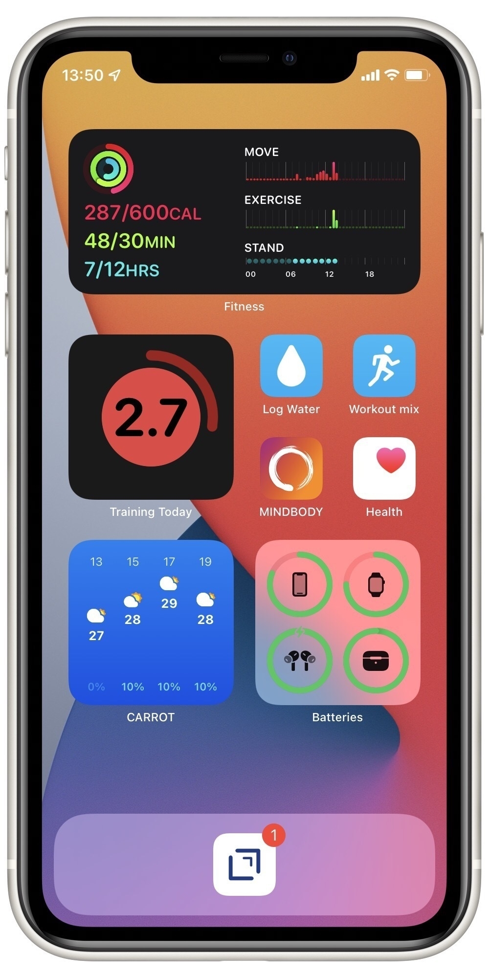
Fitness
The Fitness Home Screen is mostly an experiment. I spend the vast majority of my time in one of the other two Focus Modes, so I’m not yet convinced that I need any other Home Screens.
Regardless, this one has the Fitness widget at the top for seemingly obvious reasons.
The middle row has the Training Today widget to help keep me honest about rest. And then a cluster of icons on the right. The only one that is non-standard is “Workout mix”, which is just a Shortcut to launch a good playlist in Apple Music.
The bottom row has Carrot Weather to make sure I’m not about to get rained on when heading out for a run. I’ve also added the Batteries widget there to make sure my Apple Watch and AirPods are ready for action.
I’ve set up Personal Automations to automatically switch between my Personal and Work Home Screens at 8:45 and 17:30. I’ve found these good reminders to keep my work activities within reasonable office hours. Starting a Workout automatically switches to the Fitness Home Screen.
There’s almost endless scope for fiddling with these. So, by writing them here, I’m adding some accountability to just stop that and use them for a while before making further changes.
I like using Bookmarks as a read-it-later service and the highlighting feature is great for quickly blogging excerpts from articles. For longer-term storage, though, and integration with the rest of my notes, it is much better to have the content of the highlights stored within Notes.
So, here’s a Shortcut Micro.blog Highlights to Notes that does exactly this. The Shortcut checks first to see if the highlight is already captured in a note to prevent duplication. It also checks to see if there’s already a note for the webpage, just with a different highlight, and appends the highlight to that note, instead of creating a new one.
At least, that’s the idea. I’ve found these checks very unreliable. Sometimes the Shortcut finds the match and appends, and sometimes it doesn’t and creates a new one. Part of the problem seems to be that if there’s any punctuation in the content, the Notes filter fails. For example, searching for “We begin with an obstinate fact:” fails, then remove the “:” and the search work fine. I can use regular expressions to remove all punctuation, but then my notes are all mangled.
After fiddling around with this for a while, I’m just going to move along and assume it is a bug in the Notes actions for Shortcuts. Perhaps not a fair conclusion. The worst case is that I get one note per highlight, rather than just one note per article, and sporadically a note is duplicated. This isn’t so bad, and debugging Shortcuts can be a nuisance. Given this, the Shortcut is likely better used in an empty Notes folder, that is, delete all the previously downloaded Highlights first.
Here’s what I’ve identified so far. Many of the approaches and features that I’m using in these use cases are readily available in other apps and often Notes is not the most efficient choice. Now that I’ve documented these use cases, I’d like to use them to assess alternative apps.
Meeting notes
Thanks to Timery, I know that 60% of my working time is spent in meeting. So many meetings!
For each one, I create a note to capture ideas, useful information, and tasks. I’ve automated this with a couple of Shortcuts. The one I use the most is “Start My Next Meeting”. This presents me with a list of upcoming meetings. I choose from the list and it creates a meeting note, starts a Timery timer, and opens the link to start the video call (typically Teams). The meeting note has the name of the meeting as the title, adds tags for #meeting and the Timery project, adds the date and time of the meeting, a list of attendees, and any notes from the calendar event. From this structure, I can then add notes throughout the meeting and extract any tasks into Reminders later.
I used Agenda for these sorts of notes before, which was powerful.
Daily summaries
Occasionally, I find myself at the end of a week with no clear sense of what I actually accomplished. To help with this, for the past year I’ve been recording the top three things I’ve done in a day into Day One (the 5 Minute PM template has been great for this).
To augment this, I’ve been using another Shortcut to create a Daily Work Report. This makes a note of the meetings I attended, tasks I completed, and tasks I created. These all get saved to a Daily Notes folder. I then use the day’s work report to pull out the highlights for Day One. There’s some redundancy here, though I find the process of choosing just three things for Day One is helpful.
Overall, I think that Day One is a better app for this use case.
Project notes
For each of my projects, I create a project note that states the purpose or objective of the project, key stakeholders, and timelines. Then I accumulate relevant notes and documents while making progress on the project. Creating these are also done via a simple Shortcut. I’ve experimented with using checklists for tasks in these notes, but find it isn’t as effective as my approach with MindNode and Reminders.
Once I finish a project, the associated note gets cleaned up and moved to an Archive folder to keep it out of the way.
Research
This is a rather broad category and, unlike the previous use cases, is for both work and personal notes. Much of this is capturing facts, quotes, and sources. If it is project specific, they go to the project note. Some are more generic and are kept as a standalone note. All of them get tags to help provide some structure. This is where Apple Notes ability to accept almost anything from the share sheet is powerful.
The new Quick Notes feature has been interesting for research. The ability to quickly highlight and then resurrect content on websites is great. I find actually working with the quick notes is pretty clumsy though. They have to stay in the Quick Notes folder and choosing which one to send content to can be tricky. I think there’s some great potential here and will keep experimenting.
For any webpages that I want to archive, I use another Shortcut that creates a plain-text note of the webpage along with some metadata and then adds the link to Pinboard. This has been surprisingly useful for recipes, when all I really want are the ingredients and steps, rather than the long history of the recipe’s development.
Other nice features
In addition to these use cases, there are a few nice features of Apple Notes that are worth mentioning.
As should be apparent from above, creating useful Shortcuts for Apple Notes is straightforward. In some sense, it is the Shortcuts that I’m finding really useful. Apple Notes is just the final destination for the content.
I’ve set up widgets by focus mode so that the most recent notes are shown on my Home Screen in the right context. These are restricted to a particular folder and sorted by date modified.
The formatting options are comprehensive, including table support.
I think I like the feature where checking off tasks moves them to the bottom of the list. Most of the time, this is what I want.
The iCloud web app is convenient for using notes on my Windows work PC. Unfortunately, I’ve found the syncing to be rather unreliable here, where notes just don’t show up in the web app sometimes.
I don’t share notes as often as I expected. When I do, it works really well.
Not really specific to Apple Notes, but I stole an idea from Matthew Cassinelli to aggregate all of these Notes Shortcuts into one super Shortcut that creates a list of Shortcuts to choose from.
Challenges
There are a few things that don’t work as well as they should:
Searching is too limited. In particular, you can’t narrow searches to particular folders. Most of the time I either only want to search my meeting notes or not include them. I had to set up a Shortcut that takes a search term as an input and then asks me to specify which folder to search. This should be built into the app’s search field.
Linking among notes isn’t really supported. You can sort of do this with url searches for note titles. Pretty clunky though.
Given how much I use Shortcuts for Apple Notes, it is frustrating how little you can do when creating a note. In particular, you can’t style text or add tags. Every time I use Shortcuts to create a note, the first thing I have to do is apply title and heading styles and convert any words prefixed with a # into an actual tag.
Other use cases
I’ve found a few use cases that don’t yet fit in with Apple Notes. I’m using Drafts for all of these:
Blog posts
Drafting long emails
Capturing and processing transitory texts, which Drafts is really optimized for
Restricting myself to Apple Notes was a helpful trick for crystallizing my use cases. Now that I’m three months in, I think I’ll stick with Apple Notes for a while longer. I’ve built up a good ecosystem of Shortcuts for working with the app and, of course, now have lots of content in the app.
One less account to worry about. Not that it was a big deal, but now I don’t need to know the various setup details for my personal email. Once I’ve logged into my iCloud account, my email is ready.
I’m already paying for iCloud+ and, so, might as well use this feature and save some money by not paying for separate email hosting.
I’m actively using Reminders and Notes in iCloud.com and the Mail interface there is decent, certainly better than the rudimentary one offered by my previous email host.
Setup was straightforward with clear instructions. Having said that, the only issue I had was that initiating the setup process simply didn’t work for a few weeks. I tried a couple of times a week and each time I just got a generic error. Then, for no apparent reason, one day it worked. I suspect this was just an issue with rolling out a new service.
I should point out that my email needs are very basic for this personal account. I don’t need many automated rules, tagging, or filtering. So, iCloud Mail is fine. I wouldn’t switch over my work account (even if corporate IT would allow it). I get something like 100x the email at work and need more sophisticated tools.
Besides the initial trouble with initiating the setup, everything has been working well for the past week. I’m well aware of Apple’s well-earned reputation for challenges with internet services and will be staying vigilant for at least the next few weeks. One of the great benefits of having my own domain name is the ease with which I can switch mail hosts.
Statistics Canada has a wealth of data that are essential for good public policy. Often a good third of my analytical scripts are devoted to accessing and processing data from the Statistics Canada website, which always seems like a waste of effort and good opportunity for making silly errors. So, I was keen to test out the cansimpackage for R to see how it might help. The quick answer is “very much”.
The documentation for the cansim package is thorough and doesn’t need to be repeated here. I thought it might be useful to illustrate how helpful the package can be by refactoring some earlier work that explored consumer price inflation.
These scripts always start off with downloading and extracting the relevant data file:
You need to know the url for the data. Sometimes the logic is clear and you can guess, but often that doesn’t work and you need to spelunk through the Stats Can website
To avoid downloading the file every time I run the script, there’s a test to see if the file already exists
This approach yields lots of files and folders that you need to manage, including making sure they’re ignored by version control
Using the great readr package imports the final csv file
With cansim all I need to know is the data series number:
get_cansimdownloads the right file to a temporary directory, extracts the data, and imports it as a tidyverse-compatible data frame.
The get_cansim function has some other nice features. It automatically creates a Date column with the right type, inferred from the standard REF_DATE column. And, it also creates a val_norm column that intelligently converts the VALUE column. For example, converting percentage or thousand-dollar values into standard formats.
The cansim package is a great example of a really helpful utility package that allows me to focus on analysis, rather than fiddling around with data. Definitely worth checking out if you deal with data from Statistics Canada.
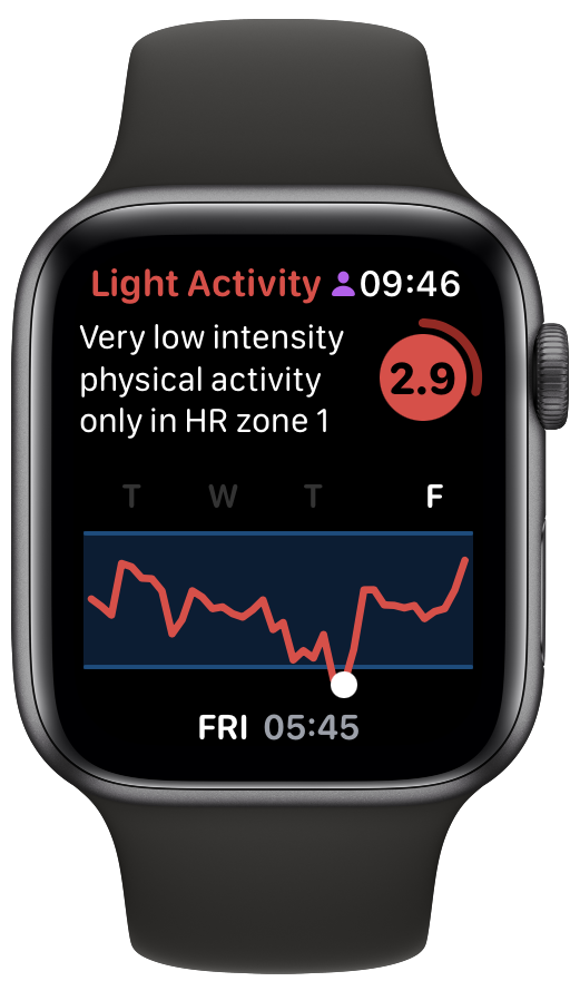
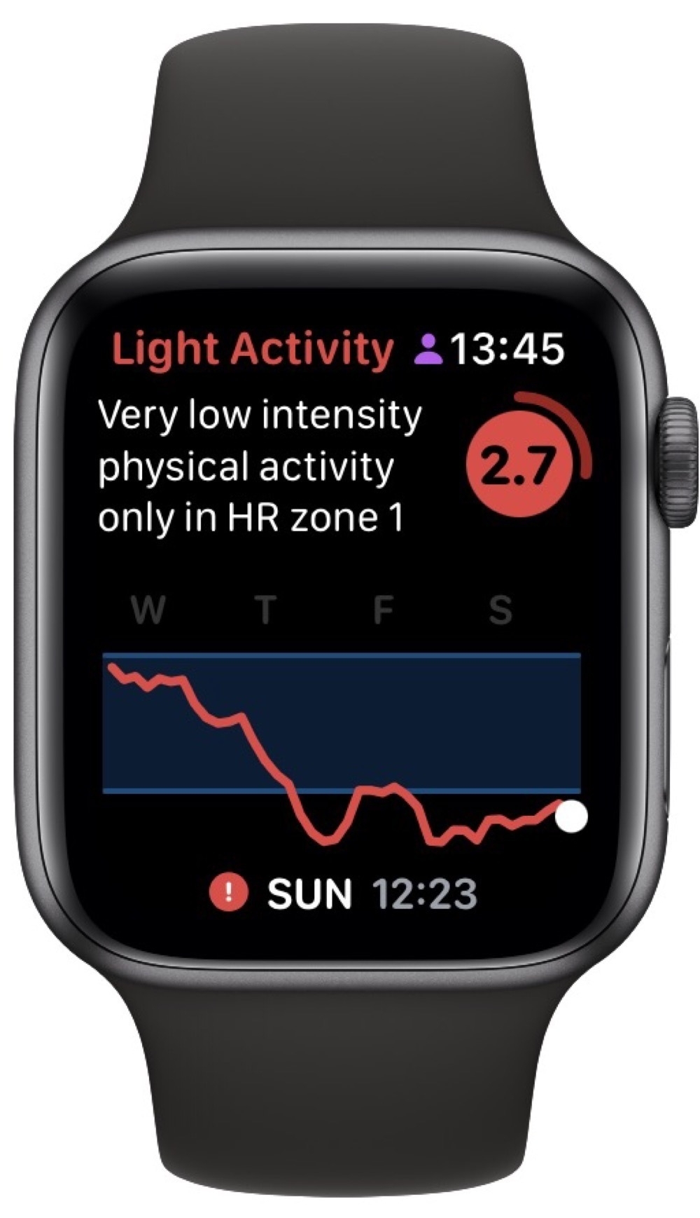
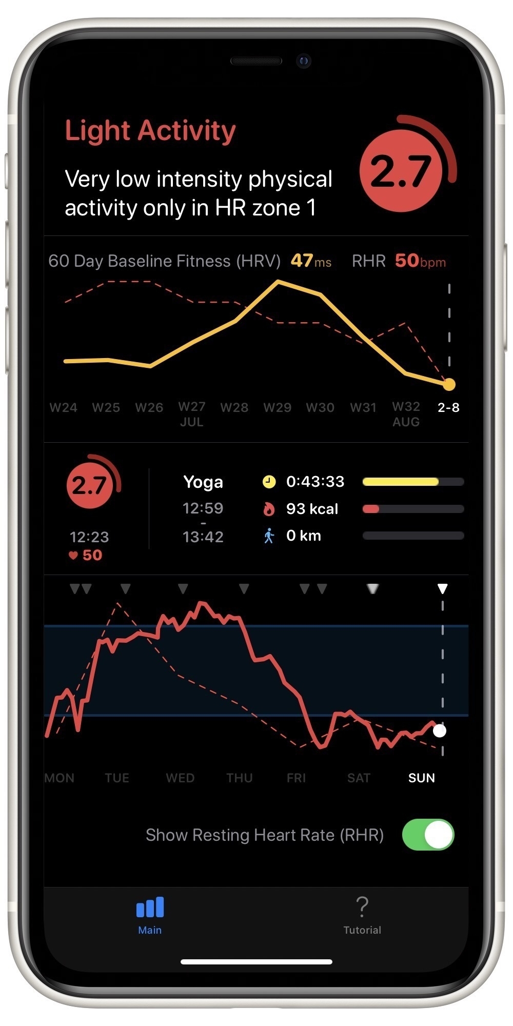
I’m trying to sequence my workouts in a more systematic way to avoid overtraining. I’ve found Training Today really helpful in determining this Readiness To Train (RTT). The app uses data collected by my Apple Watch to provide a straightforward indicator of how ambitious I should be on any particular day.
As an example, here’s today’s evaluation:
This matches how I feel 🥴. So, today was a good day for some recuperative yoga.
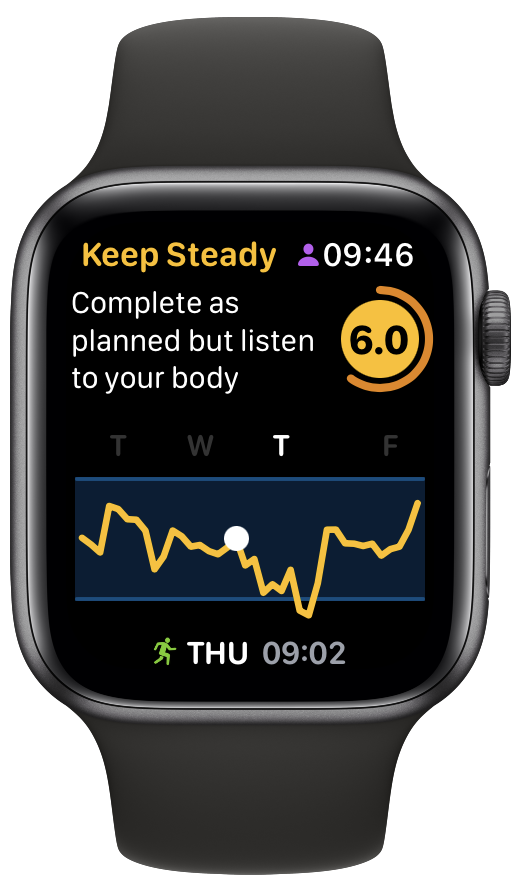
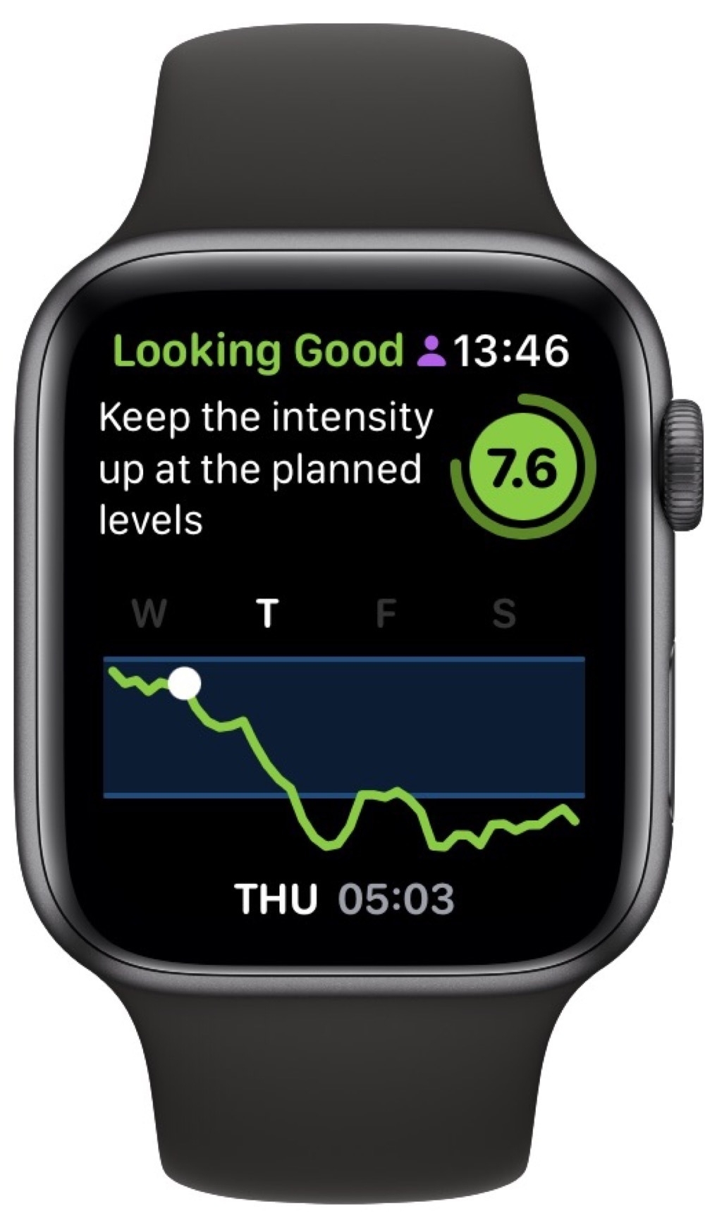
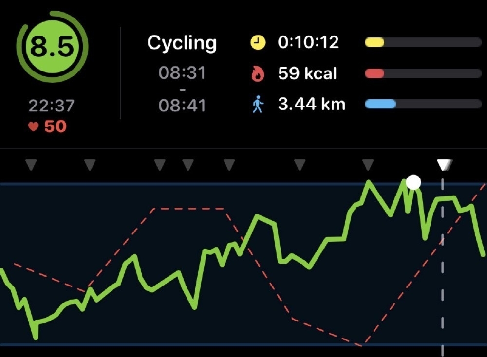
Scrolling back to Thursday, everything looked much better and I put in a good HIIT session:
Of course, the whole point of doing this is to adjust my training to match how my body is recovering. I clearly didn’t do this on Friday. Rather than catch up on some sleep, I choose to do a moderate workout and my RTT stayed on the floor. Not great, considering I’d signed up for an intense One Academy Endure Challenge on Saturday. I managed to finish, which is the main goal, but it didn’t feel good.
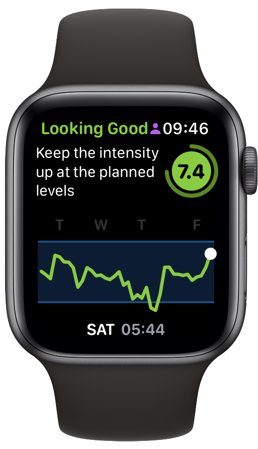
Comparing my RTT for this week’s Endure Challenge with the last one shows how this indicator can be informative:
My RTT was much higher back then and I felt really good during the challenge. This gives me comfort that RTT is actually measuring something real and actionable.
The Apple Watch screenshots shown above are part of the free version of the Training Today app. The more detailed chart above is included in a one-time in-app purchase. This gets you details like this:
And a simple widget, shown below on my fitness home screen:
I really like the focussed simplicity of Training Today, along with the straightforward one-time purchase. My Apple Watch is collecting lots of data about me and I’m glad I can use it to better manage my fitness.
In my corner of the internet, there’s a well trodden, twisted path of searching for the one true notes app. I’ve reached a fork in the path between Agenda and Craft. As I wrote earlier, I’ve been using Agenda for a while now and its date-based approach really suits my meeting-dominated work. Now, though, Craft has added calendar integration and I’m testing it out.
There are several things I really like about Craft, relative to Agenda:
Document syncing is far more reliable. This isn’t entirely Agenda’s fault. I’m restricted by corporate policy from using iCloud Documents, so have been using Dropbox sync for Agenda. I often have to wait an indeterminate, though long, time before documents sync across my devices. Craft sync has been instantaneous and very reliable.
Having access to my documents from a web browser is great. I’ll be back to working from the office on a Windows laptop soon and won’t have access to my iPad. So, web access will be important.
Performance is much better on Craft. Agenda often freezes in the middle of typing and suffers from random crashes. This could very well be something about my particular setup, though it doesn’t happen in any other apps.
On the downside, I do miss Agenda’s simplicity. Craft has lots of ways to organize notes (such as cards and subpages). Of course, you can mostly ignore this, but I like Agenda’s well-thought-through approach that didn’t require much deliberation about where to put things.
Of course, having just made this switch, Apple announced Quick Notes and I may well be back on Apple Notes in a few months.
There’s been a fair bit of discussion over on Micro.blog about podcast players recently. I’ve switched among Overcast, Castro, and Apple Podcasts players over the years and, mostly to help myself think it through (again), here are my thoughts.
For me, there are three main criteria: audio quality, episode management, and OS integration. Though, I completely understand that others may have different criteria.
Like most podcast listeners, I listen at high speed, usually around 1.5x, which can distort the audio. Apple Podcasts player is definitely the worst for this criterion. For me, Overcast’s smart speed and voice boost features give it the edge over Castro, in terms of audio quality at increased speeds.
Castro is definitely the player of choice if you subscribe to more podcasts than you can listen to. The queue management features in Castro are very good. You can replicate some of this with Overcast, but that isn’t one of the app’s main features. Apple Podcasts player doesn’t offer much in this regard. Despite listing this as a criterion, I’ve actually elevated to subscription, rather than episode, triage. I carefully curate my list of podcasts and don’t add new ones very often. Given this, Overcast’s approach is more than sufficient for me.
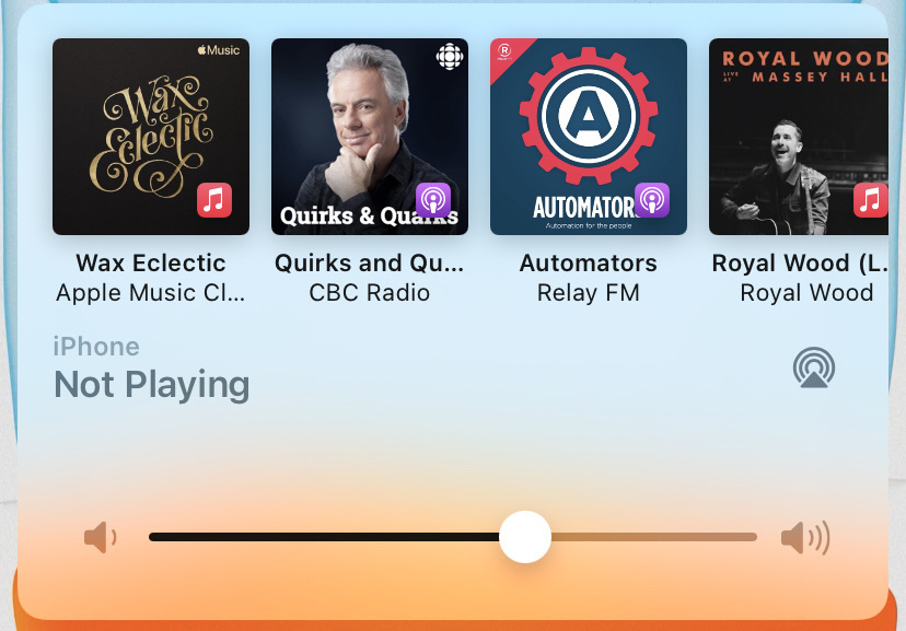
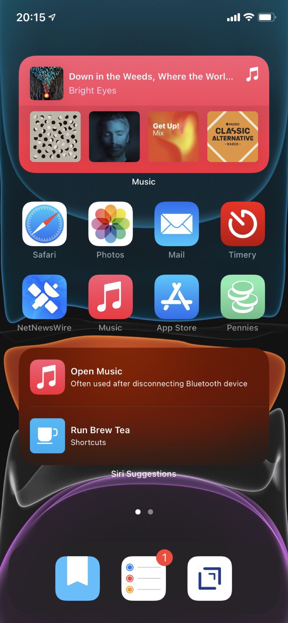
OS integration is a bit unfair, as Apple has given themselves some nice features that independent app developers aren’t able to use. Nonetheless, Apple does a good job of intermixing podcasts and music into their Siri-powered widgets in iOS and the HomePods. With my reinforced interest in less screen time and use of home screen widgets, Apple Podcasts wins out here. This may change once Overcast releases a widget.
As just one example of the integration, here’s what happens when I plug headphones into my iPhone: a selection of music playlists and podcasts appears. I use this feature a lot.
After all that, I’m using Apple Podcasts for now, mostly to take advantage of the OS integrations while I’m experimenting with a widget-based iPhone. I’m quite certain this is short term and that I’ll return to Overcast soon. In addition to the better audio quality, Overcast also has some nice refinements, like per subscription speed settings (I like to play music podcasts at 1x) and skip-forward amounts (Quirks and Quarks, for example, always has a two-minute preamble that I skip). These small refinements are typically what distinguishes the stock Apple apps from good indie apps.
I’m glad there are so many solid apps for podcast listening. Whatever your preferences, there’s sure to be one for you.
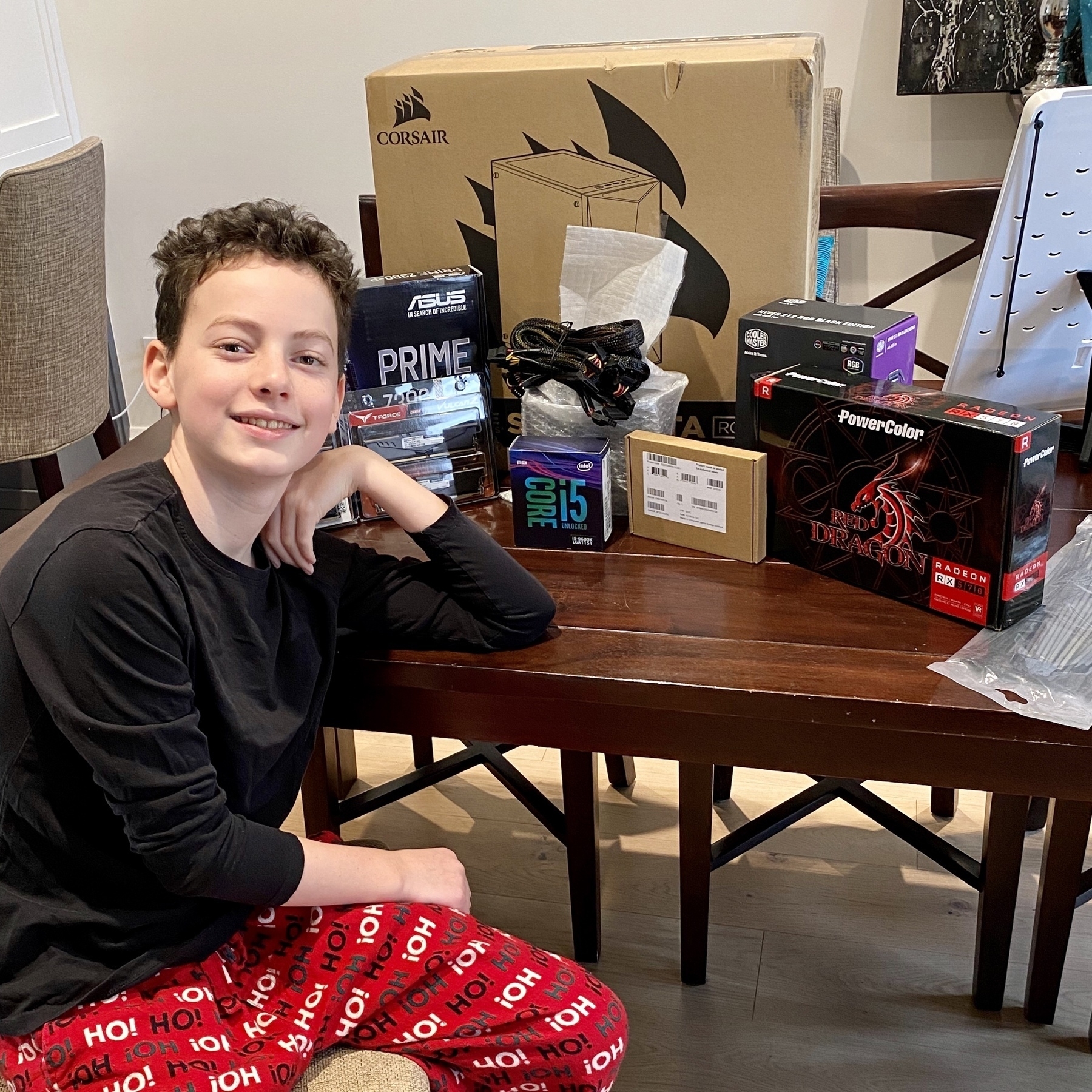
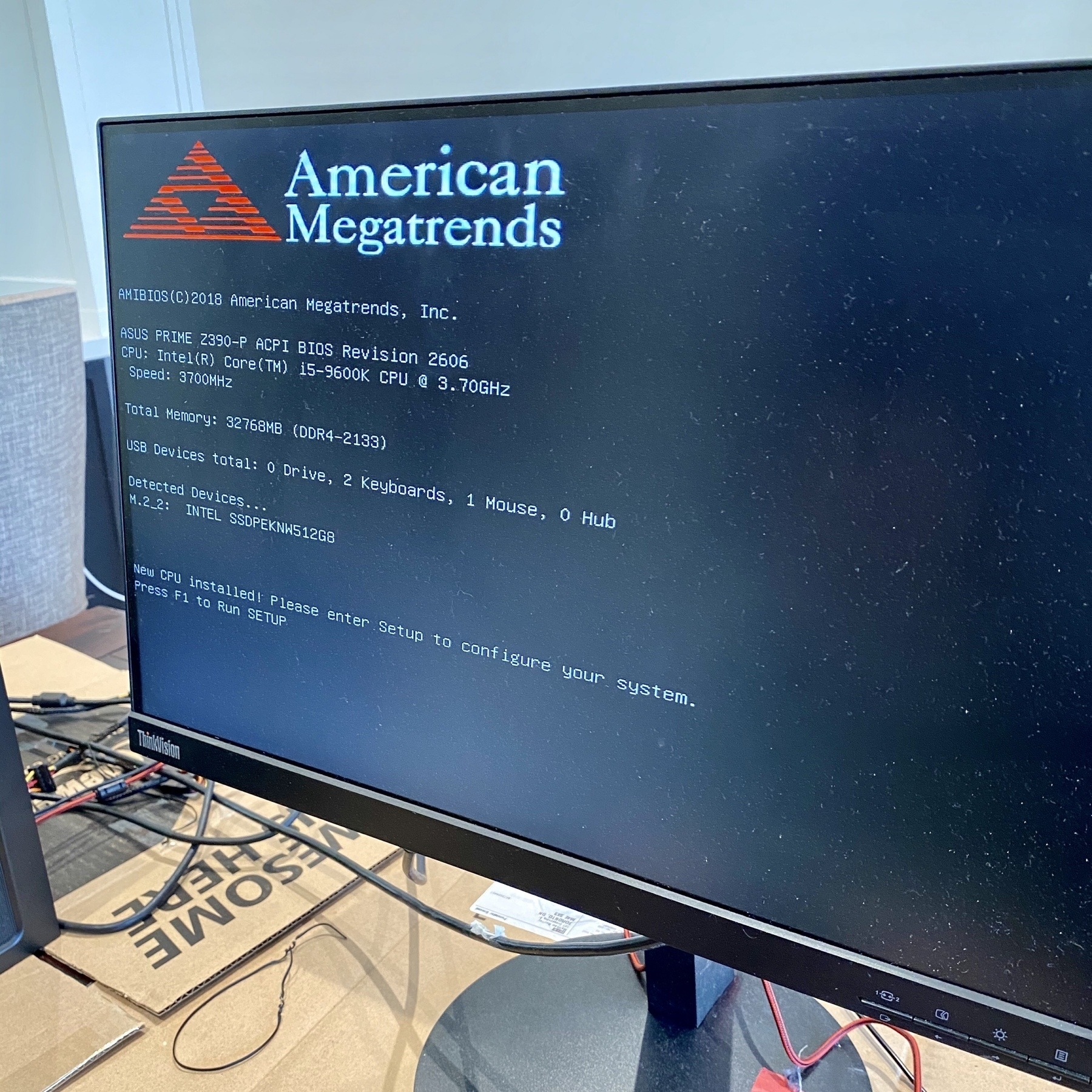
Like any 12-year old, my son is pretty keen on gaming. As an all Apple house, his options were a bit constrained. So, we decided to build a PC from components.
I’d last built a PC about 30 years ago, when I wasn’t much older than him. I remember thinking it was cool to be using a machine I’d built myself, plus as a parent it seemed like a good educational experience. I have to admit to being a bit nervous about the whole thing, as there was certainly a scenario in which we spent an entire weekend unsuccessfully trying to get a bunch of malfunctioning components to work.
After much deliberation and analysis, we ordered our parts from Newegg and everything arrived within a couple of weeks.
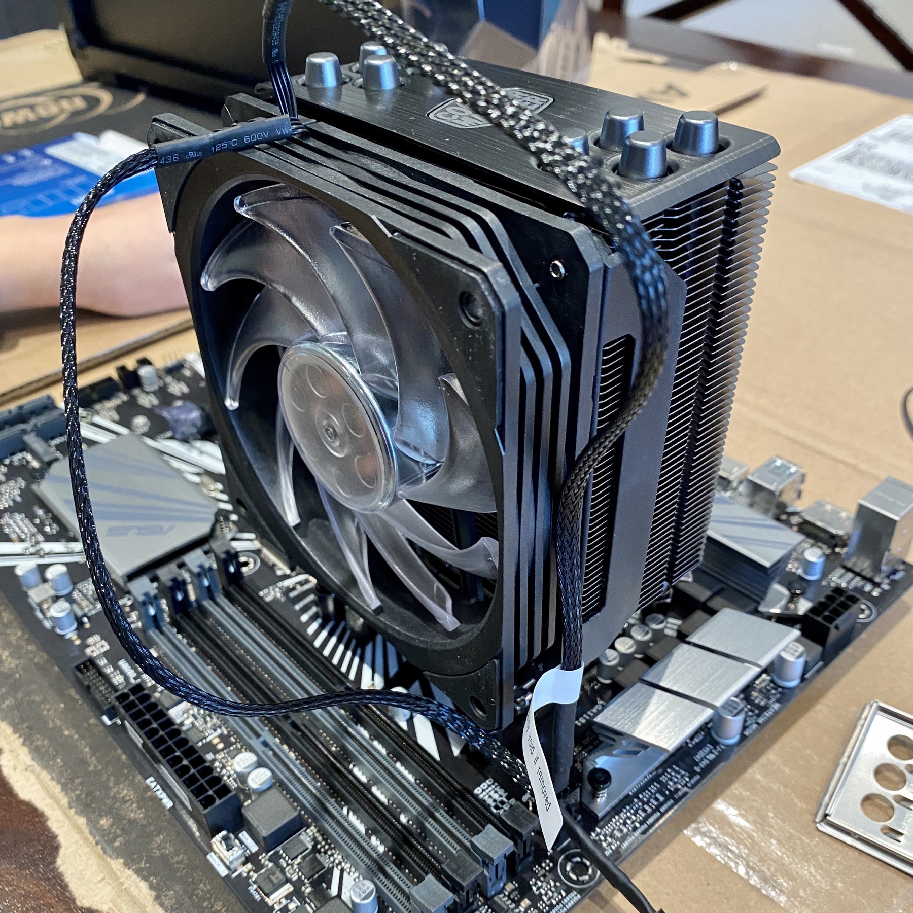
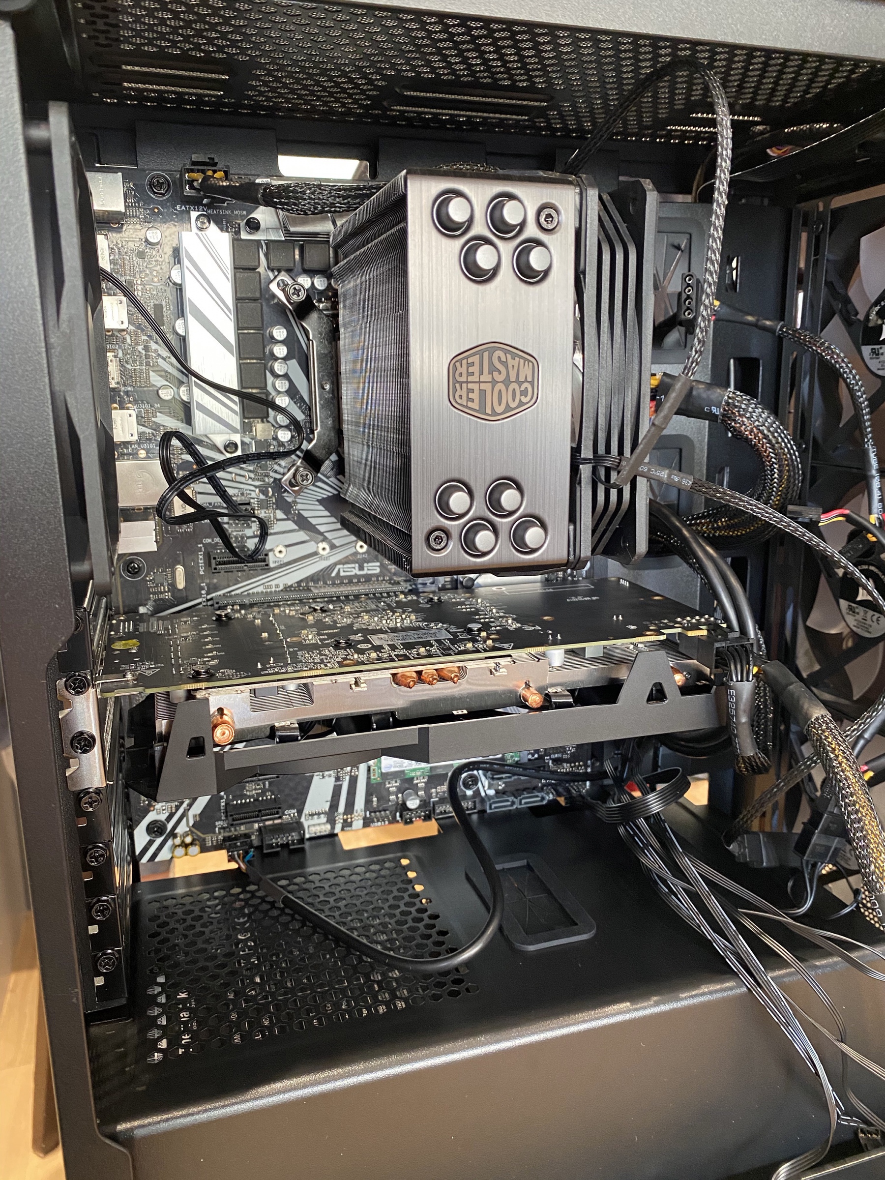
Given my initial anxiety, I was very relieved when we saw this screen. The BIOS booted up and showed that the RAM, SSD, and other components were all properly connected.
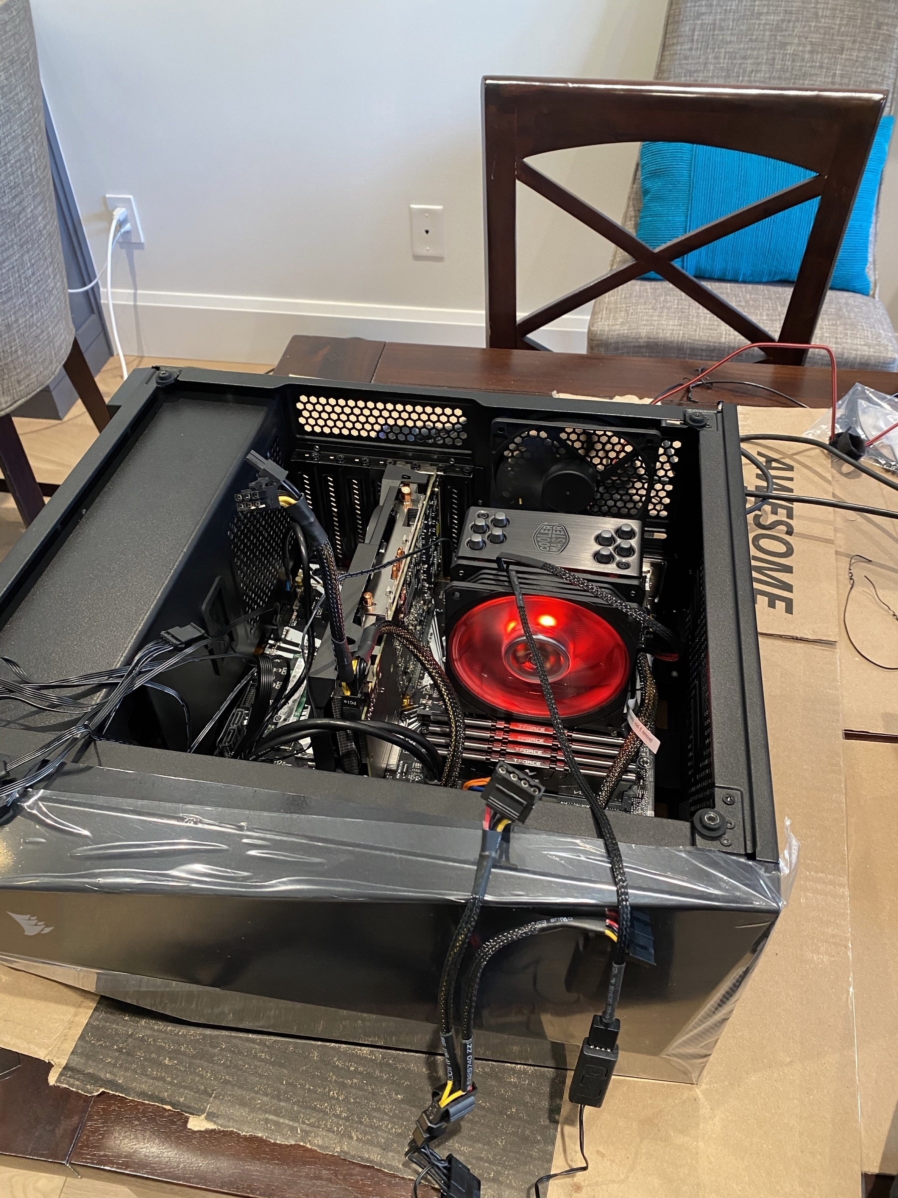
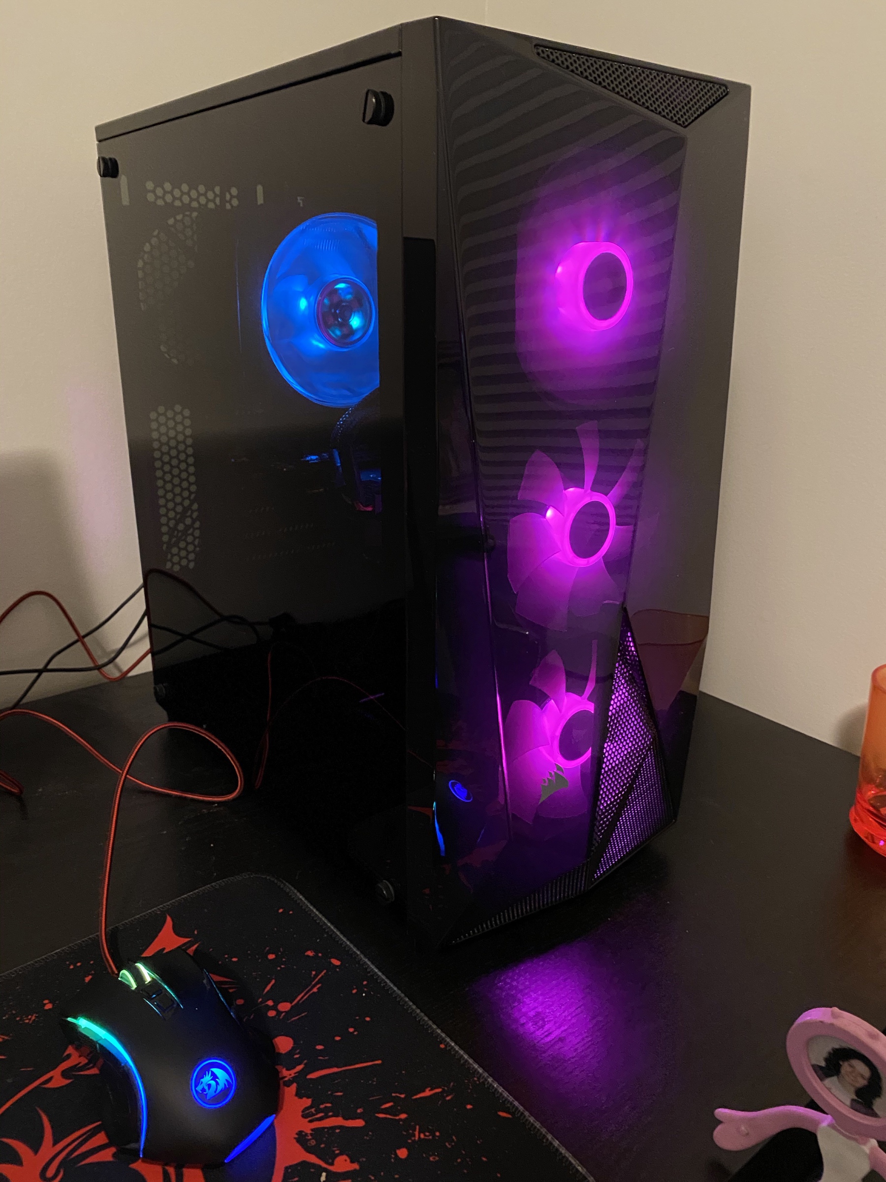
With that done, we then got to what ended up being the complicated part. Evidently part of the point of a gaming PC is to have lots of fans and lights. None of this was true when I was a kid and there were a daunting number of wires required to power the lights and fans. Sorting this out actually took a fair bit of time. But, eventually success!
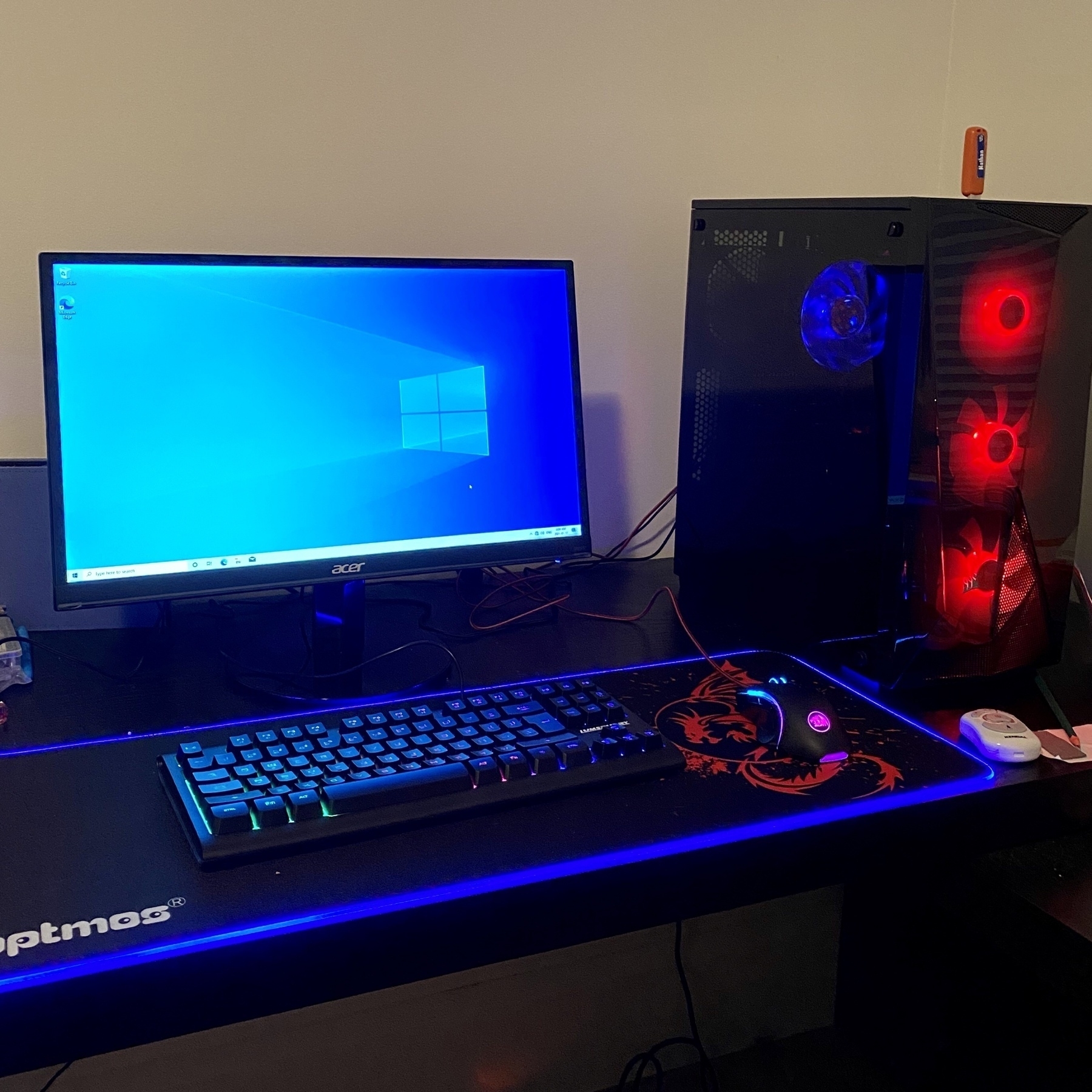
Then our last challenge, which I likely should have anticipated much sooner. We didn’t bother ordering a DVD drive, since everything is online these days. But, our Windows installation showed up as a DVD and we couldn’t create any Windows install media on our Apple devices. Fortunately, we checked in with a slightly older kid down the street and he provided us with a USB drive with the right software. With that challenge solved, we finished the project!
Not counting choosing the components online, the whole project took about 5 hours from opening the boxes to booting into Windows for the first time. I’d definitely recommend it to anyone that’s tempted and technically inclined. My son is quite excited to be using a computer that he built from parts.
Staying in touch with my team is important. So, I schedule a skip-level meeting with someone on the team each week. These informal conversations are great for getting to know everyone, finding out about new ideas, and learning about recent achievements.
Getting these organized across a couple of dozen people is logistically challenging and I’ve developed a Shortcut to automate most of the process.
Borrowing from Scotty Jackson, I have a base in AirTable with a record for each team member. I use this to store all sorts of useful information about everyone, including when we last had a skip-level meeting. The Shortcut uses this field to pull out team members that I haven’t met with in the past four months and then randomizes the list of names. Then it passes each name over to Fantastical while also incrementing the date by a week. The end result is a recurring set of weekly meetings, randomized across team members.
The hardest part of the Shortcut development was figuring out how to get the names in a random order. A big thank you to sylumer in the Automators forum for pointing out that the Files action can randomly sort any list, not just lists of files.
I’m not sharing the Shortcut here, since the implementation is very specific to my needs. Rather, I’m sharing some of the thinking behind the code, since I think that it demonstrates the general utility of something like Shortcuts for managing routine tasks with just a small amount of upfront effort.
Inspired by Coretex, I’m declaring Tangible as my theme for 2021.
I’ve chosen this theme because I want to spend less time looking at a screen and more time with “tangible stuff”. I’m sure that this is a common sentiment and declaring this theme will keep me focused on improvements.
Since working from home with an iPad, I’m averaging about 9 hours a day with an iOS device. This isn’t just a vague estimate; Screen Time gives me to-the-minute tracking of every app I’m actively using.
I’m certainly not a Luddite! The ability of these rectangles of glass to take on so many functions and provide so much meaningful content is astounding. There’s just something unsettling about the dominant role they play.
So, a few things I plan to try:
Although I’ll continue reading ebooks, since the convenience is so great, I’ll be rotating paper books into the queue regularly.
I’ve lost my running outdoor routine. Getting that back will be a nice addition to the Zoom classes and add in some very much needed fresh air.
As a family, we’ve been enjoying playing board games on weekends, just not routinely. Making sure we play at least one game a week will be good for all of us.
My son is keen on electronics. We’re going to try assembling a gaming PC for him from components, as well as learn some basic electronics with a breadboard and Arduino.
Our dog will be excited to get out for more regular walks with especially long ones on the weekend.
I’ll be adding much of this to Streaks, an app that I’ve found really helpful for building habits. I’ll also add a “tangible” tag to my time tracker to quantify the shift.
My hope is that I can find the right balance of screen time and tangible activities with intention.
MindNode is indispensable to my workflow. My main use for it is in tracking all of my projects and tasks, supported by MindNode’s Reminders integration. I can see all of my projects, grouped by areas of focus, simultaneously which is great for weekly reviews and for prioritizing my work.
I’ve also found it really helpful for sketching out project plans. I can get ideas out of my head easily with quick entry and then drag and drop nodes to explore connections. Seeing connections among items and rearranging them really brings out the critical elements.
MindNode’s design is fantastic and the app makes it really easy to apply styles across nodes. The relatively recent addition of tags has been great too. Overall, one of my most used apps.
I’m very excited to be recruiting for a Data Governance Sponsor to join my team and help enhance the use of good data analytics in our decisions at Metrolinx.
I’m looking for someone that enjoys telling compelling stories with data and has a passion for collaborating to build clean and reliable analytical processes. If you know someone that could fit (maybe you!), please pass along the job ad
I’ve been negligent in supporting some of my favourite apps on the App Store. In many cases, I reviewed the app a few years ago and then never refreshed my ratings. So, I’m making a new commitment to updating my reviews for apps by picking at least one each month to refresh.
First up is Fantastical. This one took a real hit when they switched to a subscription pricing model. I get the controversy with subscriptions in general. For me, Fantastical has earned a spot on my short list of apps that I support with an ongoing subscription.
And here’s my App Store review:
Fantastical is a great app and is definitely one of my top three most-used apps. Well worth the subscription price.
A few favourite features:
Integration of events and tasks into the calendar view
Access to event attachments
Automatic link detection for Teams and Zoom meetings
With the release of iOS 7, I’m reconsidering my earlier approach to the Home Screen. So far I’m trying out a fully automated first screen that uses the Smart Stack, Siri Suggestions, and Shortcut widgets. These are all automatically populated, based on anticipated use and have been quite prescient.
My second screen is all widgets with views from apps that I want to have always available. Although the dynamic content on the first screen has been really good, I do want some certainty about accessing specific content. This second screen replaces how I was using the Today View. I’m not really sure what to do with that feature anymore.
I’ve hidden all of the other screens and rely on the App Library and search to find anything else.
I still like the simplicity behind my earlier approach to the Home Screen. We’ll see if that is just what I’m used to. This new approach is worth testing out for at least a few weeks.