Commiting to a Fitness Challenge and Then Figuring Out if it is Achievable
My favourite spin studio has put on a fitness challenge for 2019. It has many components, one of which is improving your performance by 3% over six weeks. I’ve taken on the challenge and am now worried that I don’t know how reasonable this increase actually is. So, a perfect excuse to extract my metrics and perform some excessive analysis.
We start by importing a CSV file of my stats, taken from Torq’s website. We use readr for this and set the col_types in advance to specify the type for each column, as well as skip some extra columns with col_skip. I find doing this at the same time as the import, rather than later in the process, more direct and efficient. I also like the flexibility of the col_date import, where I can convert the source data (e.g., “Mon 11/02/19 - 6:10 AM”) into a format more useful for analysis (e.g., “2019-02-11”).
One last bit of clean up is to specify the instructors that have led 5 or more sessions. Later, we’ll try to identify an instructor-effect on my performance and only 5 of the 10 instructors have sufficient data for such an analysis. The forcats::fct_other function is really handy for this: it collapses several factor levels together into one “Other” level.
Lastly, I set the challenge_start_date variable for use later on.
col_types = cols(
  Date = col_date(format = "%a %d/%m/%y - %H:%M %p"),
  Ride = col_skip(),
  Instructor = col_character(),
  Spot = col_skip(),
  `Avg RPM` = col_skip(),
  `Max RPM` = col_skip(),
  `Avg Power` = col_double(),
  `Max Power` = col_double(),
  `Total Energy` = col_double(),
  `Dist. (Miles)` = col_skip(),
  Cal. = col_skip(),
  `Class Rank` = col_skip()
)
main_instructors <- c("Tanis", "George", "Charlotte", "Justine", "Marawan") # 5 or more sessions
data <- readr::read_csv("torq_data.csv", col_types = col_types) %>%
  tibbletime::as_tbl_time(index = Date) %>%
  dplyr::rename(avg_power    = `Avg Power`,
                max_power    = `Max Power`,
                total_energy = `Total Energy`) %>%
  dplyr::mutate(Instructor =
                  forcats::fct_other(Instructor, keep = main_instructors))
challenge_start_date <- lubridate::as_date("2019-01-01")
head(data)
## # A time tibble: 6 x 5
## # Index: Date
## Date Instructor avg_power max_power total_energy
##
## 1 2019-02-11 Justine 234 449 616
## 2 2019-02-08 George 221 707 577
## 3 2019-02-04 Justine 230 720 613
## 4 2019-02-01 George 220 609 566
## 5 2019-01-21 Justine 252 494 623
## 6 2019-01-18 George 227 808 590 To start, we just plot the change in average power over time. Given relatively high variability from class to class, we add a smoothed line to show the overall trend. We also mark the point where the challenge starts with a red line.
ggplot2::ggplot(data, aes(x = Date, y = avg_power)) +
  ggplot2::geom_point() +
  ggplot2::geom_line() +
  geom_smooth(method = "loess") +
  ggplot2::ylab("Average power") +
  ggplot2::geom_vline(xintercept = challenge_start_date, col = "red")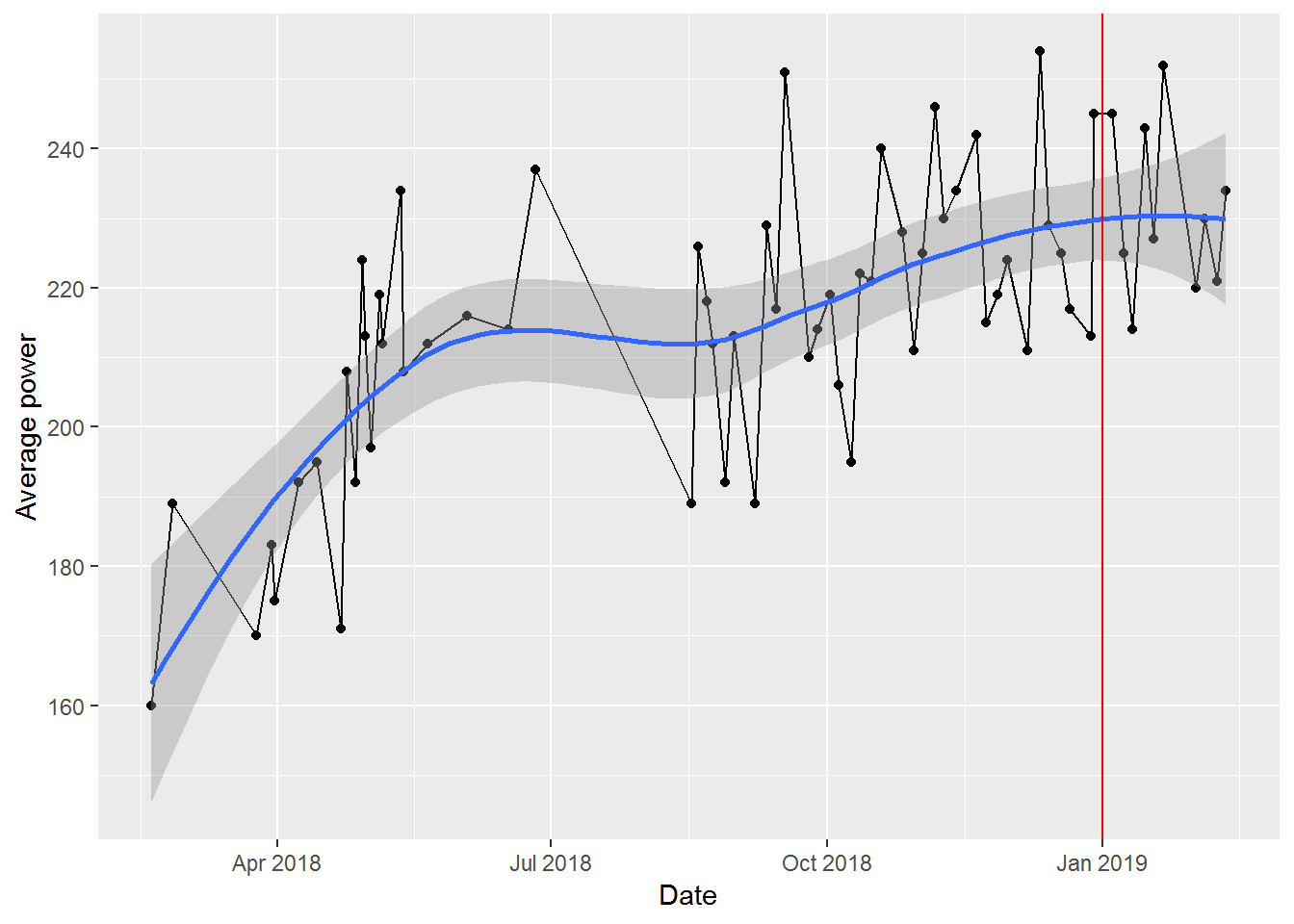
Overall, looks like I made some steady progress when I started, plateaued in the Summer (when I didn’t ride as often), and then started a slow, steady increase in the Fall. Unfortunately for me, it also looks like I started to plateau in my improvement just in time for the challenge.
We’ll start a more formal analysis by just testing to see what my average improvement is over time.
time_model <- lm(avg_power ~ Date, data = data)
summary(time_model)
##
## Call:
## lm(formula = avg_power ~ Date, data = data)
##
## Residuals:
## Min 1Q Median 3Q Max
## -30.486 -11.356 -1.879 11.501 33.838
##
## Coefficients:
## Estimate Std. Error t value Pr(>|t|)
## (Intercept) -2.032e+03 3.285e+02 -6.186 4.85e-08 ***
## Date 1.264e-01 1.847e-02 6.844 3.49e-09 ***
## ---
## Signif. codes: 0 '***' 0.001 '**' 0.01 '*' 0.05 '.' 0.1 ' ' 1
##
## Residual standard error: 15.65 on 64 degrees of freedom
## Multiple R-squared: 0.4226, Adjusted R-squared: 0.4136
## F-statistic: 46.85 on 1 and 64 DF, p-value: 3.485e-09Based on this, we can see that my performance is improving over time and the R2 is decent. But, interpreting the coefficient for time isn’t entirely intuitive and isn’t really the point of the challenge. The question is: how much higher is my average power during the challenge than before? For that, we’ll set up a “dummy variable” based on the date of the class. Then we use dplyr to group by this variable and estimate the mean of the average power in both time periods.
data %<>%
  dplyr::mutate(in_challenge = ifelse(Date > challenge_start_date, 1, 0))
(change_in_power <- data %>%
  dplyr::group_by(in_challenge) %>%
  dplyr::summarize(mean_avg_power = mean(avg_power)))
## # A tibble: 2 x 2
## in_challenge mean_avg_power
##
## 1 0 213.
## 2 1 231. So, I’ve improved from an average power of 213 to 231 for a improvement of 8%. A great relief: I’ve exceeded the target!
Of course, having gone to all of this (excessive?) trouble, now I’m interested in seeing if the instructor leading the class has a significant impact on my results. I certainly feel as if some instructors are harder than others. But, is this supported by my actual results? As always, we start with a plot to get a visual sense of the data.
ggplot2::ggplot(data, aes(x = Date, y = avg_power)) +
  ggplot2::geom_point() +
  ggplot2::geom_line() +
  ggplot2::geom_smooth(method = "lm", se = FALSE) +
  ggplot2::facet_wrap(~Instructor) +
  ggplot2::ylab("Average power")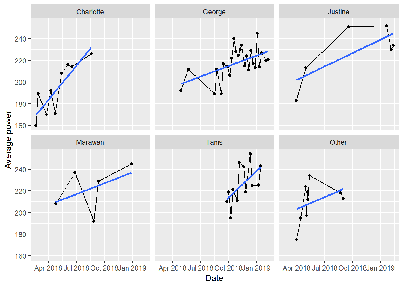
There’s a mix of confirmation and rejection of my expectations here:
- Charlotte got me started and there’s a clear trend of increasing power as I figure out the bikes and gain fitness
- George’s class is always fun, but my progress isn’t as high as I’d like (indicated by the shallower slope). This is likely my fault though: George’s rides are almost always Friday morning and I’m often tired by then and don’t push myself as hard as I could
- Justine hasn’t led many of my classes, but my two best results are with her. That said, my last two rides with her haven’t been great
- Marawan’s classes always feel really tough. He’s great at motivation and I always feel like I’ve pushed really hard in his classes. You can sort of see this with the relatively higher position of the best fit line for his classes. But, I also had one really poor class with him. This seems to coincide with some poor classes with both Tanis and George though. So, I was likely a bit sick then. Also, for Marawan, I’m certain I’ve had more classes with him (each one is memorably challenging), as he’s substituted for other instructors several times. Looks like Torq’s tracker doesn’t adjust the name of the instructor to match this substitution though
- Tanis’ classes are usually tough too. She’s relentless about increasing resistance and looks like I was improving well with her
- Other isn’t really worth describing in any detail, as it is a mix of 5 other instructors each with different styles.
Having eye-balled the charts. Let’s now look at a statistical model that considers just instructors.
instructor_model <- update(time_model, . ~ Instructor)
summary(instructor_model)
##
## Call:
## lm(formula = avg_power ~ Instructor, data = data)
##
## Residuals:
## Min 1Q Median 3Q Max
## -44.167 -10.590 0.663 13.540 32.000
##
## Coefficients:
## Estimate Std. Error t value Pr(>|t|)
## (Intercept) 194.000 6.123 31.683 < 2e-16 ***
## InstructorGeorge 23.840 7.141 3.339 0.001451 **
## InstructorJustine 33.167 9.682 3.426 0.001112 **
## InstructorMarawan 28.200 10.246 2.752 0.007817 **
## InstructorTanis 31.833 8.100 3.930 0.000222 ***
## InstructorOther 15.667 8.660 1.809 0.075433 .
## ---
## Signif. codes: 0 '***' 0.001 '**' 0.01 '*' 0.05 '.' 0.1 ' ' 1
##
## Residual standard error: 18.37 on 60 degrees of freedom
## Multiple R-squared: 0.2542, Adjusted R-squared: 0.1921
## F-statistic: 4.091 on 5 and 60 DF, p-value: 0.002916Each of the named instructors has a significant, positive effect on my average power. However, the overall R2 is much less than the model that considered just time. So, our next step is to consider both together.
time_instructor_model <- update(time_model, . ~ . + Instructor)
summary(time_instructor_model)
##
## Call:
## lm(formula = avg_power ~ Date + Instructor, data = data)
##
## Residuals:
## Min 1Q Median 3Q Max
## -31.689 -11.132 1.039 10.800 26.267
##
## Coefficients:
## Estimate Std. Error t value Pr(>|t|)
## (Intercept) -2332.4255 464.3103 -5.023 5.00e-06 ***
## Date 0.1431 0.0263 5.442 1.07e-06 ***
## InstructorGeorge -2.3415 7.5945 -0.308 0.759
## InstructorJustine 10.7751 8.9667 1.202 0.234
## InstructorMarawan 12.5927 8.9057 1.414 0.163
## InstructorTanis 3.3827 8.4714 0.399 0.691
## InstructorOther 12.3270 7.1521 1.724 0.090 .
## ---
## Signif. codes: 0 '***' 0.001 '**' 0.01 '*' 0.05 '.' 0.1 ' ' 1
##
## Residual standard error: 15.12 on 59 degrees of freedom
## Multiple R-squared: 0.5034, Adjusted R-squared: 0.4529
## F-statistic: 9.969 on 6 and 59 DF, p-value: 1.396e-07anova(time_instructor_model, time_model)## Analysis of Variance Table
##
## Model 1: avg_power ~ Date + Instructor
## Model 2: avg_power ~ Date
## Res.Df RSS Df Sum of Sq F Pr(>F)
## 1 59 13481
## 2 64 15675 -5 -2193.8 1.9202 0.1045This model has the best explanatory power so far and increases the coefficient for time slightly. This suggests that controlling for instructor improves the time signal. However, when we add in time, none of the individual instructors are significantly different from each other. My interpretation of this is that my overall improvement over time is much more important than which particular instructor is leading the class. Nonetheless, the earlier analysis of the instructors gave me some insights that I can use to maximize the contribution each of them makes to my overall progress. When comparing these models with an ANOVA though, we find that there isn’t a significant difference between them.
The last model to try is to look for a time by instructor interaction.
time_instructor_interaction_model <- update(time_model, . ~ . * Instructor)
summary(time_instructor_interaction_model)
##
## Call:
## lm(formula = avg_power ~ Date + Instructor + Date:Instructor,
## data = data)
##
## Residuals:
## Min 1Q Median 3Q Max
## -31.328 -9.899 0.963 10.018 26.128
##
## Coefficients:
## Estimate Std. Error t value Pr(>|t|)
## (Intercept) -5.881e+03 1.598e+03 -3.680 0.000540 ***
## Date 3.442e-01 9.054e-02 3.801 0.000368 ***
## InstructorGeorge 4.225e+03 1.766e+03 2.393 0.020239 *
## InstructorJustine 3.704e+03 1.796e+03 2.062 0.044000 *
## InstructorMarawan 4.177e+03 2.137e+03 1.955 0.055782 .
## InstructorTanis 1.386e+03 2.652e+03 0.523 0.603313
## InstructorOther 3.952e+03 2.321e+03 1.703 0.094362 .
## Date:InstructorGeorge -2.391e-01 9.986e-02 -2.394 0.020149 *
## Date:InstructorJustine -2.092e-01 1.016e-01 -2.059 0.044291 *
## Date:InstructorMarawan -2.357e-01 1.207e-01 -1.953 0.056070 .
## Date:InstructorTanis -7.970e-02 1.492e-01 -0.534 0.595316
## Date:InstructorOther -2.231e-01 1.314e-01 -1.698 0.095185 .
## ---
## Signif. codes: 0 '***' 0.001 '**' 0.01 '*' 0.05 '.' 0.1 ' ' 1
##
## Residual standard error: 14.86 on 54 degrees of freedom
## Multiple R-squared: 0.5609, Adjusted R-squared: 0.4715
## F-statistic: 6.271 on 11 and 54 DF, p-value: 1.532e-06anova(time_model, time_instructor_interaction_model)## Analysis of Variance Table
##
## Model 1: avg_power ~ Date
## Model 2: avg_power ~ Date + Instructor + Date:Instructor
## Res.Df RSS Df Sum of Sq F Pr(>F)
## 1 64 15675
## 2 54 11920 10 3754.1 1.7006 0.1044We can see that there are some significant interactions, meaning that the slope of improvement over time does differ by instructor. Before getting too excited though, an ANOVA shows that this model isn’t any better than the simple model of just time. There’s always a risk with trying to explain main effects (like time) with interactions. The story here is really that we need more data to tease out the impacts of the instructor by time effect.
The last point to make is that we’ve focused so far on the average power, since that’s the metric for this fitness challenge. There could be interesting interactions among average power, maximum power, RPMs, and total energy, each of which is available in these data. I’ll return to that analysis some other time.
In the interests of science, I’ll keep going to these classes, just so we can figure out what impact instructors have on performance. In the meantime, looks like I’ll succeed with at least this component of the fitness challenge and I have the stats to prove it.