Spatial analysis of votes in Toronto
This is a “behind the scenes” elaboration of the geospatial analysis in our recent post on evaluating our predictions for the 2018 mayoral election in Toronto. This was my first, serious use of the new sf package for geospatial analysis. I found the package much easier to use than some of my previous workflows for this sort of analysis, especially given its integration with the tidyverse.
We start by downloading the shapefile for voting locations from the City of Toronto’s Open Data portal and reading it with the read_sf function. Then, we pipe it to st_transform to set the appropriate projection for the data. In this case, this isn’t strictly necessary, since the shapefile is already in the right projection. But, I tend to do this for all shapefiles to avoid any oddities later.
download.file("http://opendata.toronto.ca/gcc/voting_location_2018_wgs84.zip",
                destfile = "data-raw/voting_location_2018_wgs84.zip", quiet = TRUE)
unzip("data-raw/voting_location_2018_wgs84.zip", exdir="data-raw/voting_location_2018_wgs84")
toronto_locations <- sf::read_sf("data-raw/voting_location_2018_wgs84",
                                 layer = "VOTING_LOCATION_2018_WGS84") %>%
  sf::st_transform(crs = "+init=epsg:4326")
toronto_locations
## Simple feature collection with 1700 features and 13 fields
## geometry type:  POINT
## dimension:      XY
## bbox:           xmin: -79.61937 ymin: 43.59062 xmax: -79.12531 ymax: 43.83052
## epsg (SRID):    4326
## proj4string:    +proj=longlat +datum=WGS84 +no_defs
## # A tibble: 1,700 x 14
##    POINT_ID FEAT_CD FEAT_C_DSC PT_SHRT_CD PT_LNG_CD POINT_NAME VOTER_CNT
##       <dbl> <chr>   <chr>      <chr>      <chr>     <chr>          <int>
##  1    10190 P       Primary    056        10056     <NA>              37
##  2    10064 P       Primary    060        10060     <NA>             532
##  3    10999 S       Secondary  058        10058     Malibu           661
##  4    11342 P       Primary    052        10052     <NA>            1914
##  5    10640 P       Primary    047        10047     The Summit       956
##  6    10487 S       Secondary  061        04061     White Eag…        51
##  7    11004 P       Primary    063        04063     Holy Fami…      1510
##  8    11357 P       Primary    024        11024     Rosedale …      1697
##  9    12044 P       Primary    018        05018     Weston Pu…      1695
## 10    11402 S       Secondary  066        04066     Elm Grove…        93
## # ... with 1,690 more rows, and 7 more variables: OBJECTID <dbl>,
## #   ADD_FULL <chr>, X <dbl>, Y <dbl>, LONGITUDE <dbl>, LATITUDE <dbl>,
## #   geometry <POINT [°]>
The file has 1700 rows of data across 14 columns. The first 13 columns are data within the original shapefile. The last column is a list column that is added by sf and contains the geometry of the location. This specific design feature is what makes an sf object work really well with the rest of the tidyverse: the geographical details are just a column in the data frame. This makes the data much easier to work with than in other approaches, where the data is contained within an [@data](https://micro.blog/data) slot of an object.
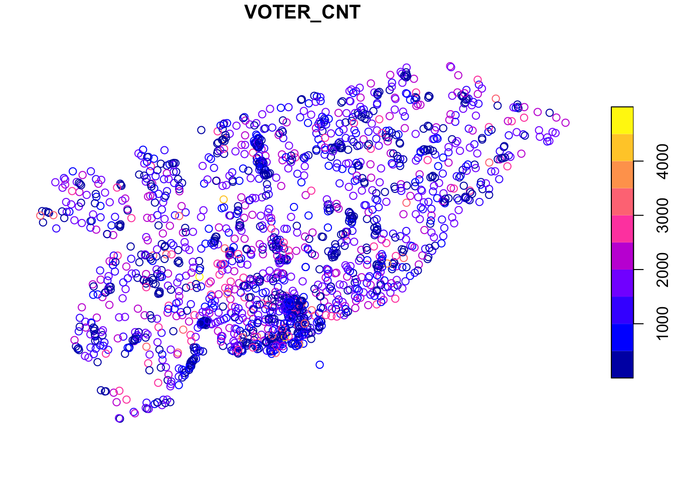
Plotting the data is straightforward, since sf objects have a plot function. Here’s an example where we plot the number of voters (VOTER_CNT) at each location. If you squint just right, you can see the general outline of Toronto in these points.
What we want to do next is use the voting location data to aggregate the votes cast at each location into census tracts. This then allows us to associate census characteristics (like age and income) with the pattern of votes and develop our statistical relationships for predicting voter behaviour.
We’ll split this into several steps. The first is downloading and reading the census tract shapefile.
download.file("http://www12.statcan.gc.ca/census-recensement/2011/geo/bound-limit/files-fichiers/gct_000b11a_e.zip",
                destfile = "data-raw/gct_000b11a_e.zip", quiet = TRUE)
unzip("data-raw/gct_000b11a_e.zip", exdir="data-raw/gct")
census_tracts <- sf::read_sf("data-raw/gct", layer = "gct_000b11a_e") %>%
  sf::st_transform(crs = "+init=epsg:4326")
Now that we have it, all we really want are the census tracts in Toronto (the shapefile includes census tracts across Canada). We achieve this by intersecting the Toronto voting locations with the census tracts using standard R subsetting notation.
to_census_tracts <- census_tracts[toronto_locations,]
And, we can plot it to see how well the intersection worked. This time we’ll plot the CTUID, which is the unique identifier for each census tract. This doesn’t mean anything in this context, but adds some nice colour to the plot.
plot(to_census_tracts["CTUID"])
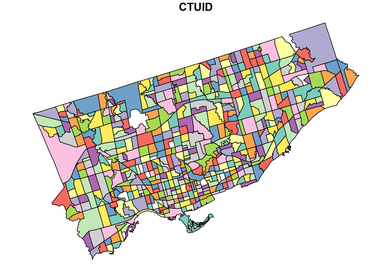
Now you can really see the shape of Toronto, as well as the size of each census tract.
Next we need to manipulate the voting data to get votes received by major candidates in the 2018 election. We take these data from the toVotes package and arbitrarily set the threshold for major candidates to receiving at least 100,000 votes. This yields our two main candidates: John Tory and Jennifer Keesmaat.
major_candidates <- toVotes %>%
  dplyr::filter(year == 2018) %>%
  dplyr::group_by(candidate) %>%
  dplyr::summarise(votes = sum(votes)) %>%
  dplyr::filter(votes > 100000) %>%
  dplyr::select(candidate)
major_candidates
## # A tibble: 2 x 1
##   candidate
##   <chr>
## 1 Keesmaat Jennifer
## 2 Tory John
Given our goal of aggregating the votes received by each candidate into census tracts, we need a data frame that has each candidate in a separate column. We start by joining the major candidates table to the votes table. In this case, we also filter the votes to 2018, since John Tory has been a candidate in more than one election. Then we use the tidyr package to convert the table from long (with one candidate column) to wide (with a column for each candidate).
spread_votes <- toVotes %>%
  tibble::as.tibble() %>%
  dplyr::filter(year == 2018) %>%
  dplyr::right_join(major_candidates) %>%
  dplyr::select(-type, -year) %>%
  tidyr::spread(candidate, votes)
spread_votes
## # A tibble: 1,800 x 4
##     ward  area `Keesmaat Jennifer` `Tory John`
##    <int> <int>               <dbl>       <dbl>
##  1     1     1                  66         301
##  2     1     2                  72         376
##  3     1     3                  40         255
##  4     1     4                  24         161
##  5     1     5                  51         211
##  6     1     6                  74         372
##  7     1     7                  70         378
##  8     1     8                  10          77
##  9     1     9                  11          82
## 10     1    10                  12          76
## # ... with 1,790 more rows
Our last step before finally aggregating to census tracts is to join the spread_votes table with the toronto_locations data. This requires pulling the ward and area identifiers from the PT_LNG_CD column of the toronto_locations data frame which we do with some stringr functions. While we’re at it, we also update the candidate names to just surnames.
to_geo_votes <- toronto_locations %>%
  dplyr::mutate(ward = as.integer(stringr::str_sub(PT_LNG_CD, 1, 2)),
                area = as.integer(stringr::str_sub(PT_LNG_CD, -3, -1))) %>%
  dplyr::left_join(spread_votes) %>%
  dplyr::select(`Keesmaat Jennifer`, `Tory John`) %>%
  dplyr::rename(Keesmaat = `Keesmaat Jennifer`, Tory = `Tory John`)
to_geo_votes
## Simple feature collection with 1700 features and 2 fields
## geometry type:  POINT
## dimension:      XY
## bbox:           xmin: -79.61937 ymin: 43.59062 xmax: -79.12531 ymax: 43.83052
## epsg (SRID):    4326
## proj4string:    +proj=longlat +datum=WGS84 +no_defs
## # A tibble: 1,700 x 3
##    Keesmaat  Tory             geometry
##       <dbl> <dbl>          <POINT [°]>
##  1       55   101 (-79.40225 43.63641)
##  2       43    53  (-79.3985 43.63736)
##  3       61    89 (-79.40028 43.63664)
##  4      296   348 (-79.39922 43.63928)
##  5      151   204 (-79.40401 43.64293)
##  6        2    11 (-79.43941 43.63712)
##  7      161   174 (-79.43511 43.63869)
##  8      221   605  (-79.38188 43.6776)
##  9       68   213 (-79.52078 43.70176)
## 10        4    14 (-79.43094 43.64027)
## # ... with 1,690 more rows
Okay, we’re finally there. We have our census tract data in to_census_tracts and our voting data in to_geo_votes. We want to aggregate the votes into each census tract by summing the votes at each voting location within each census tract. We use the aggregate function for this.
ct_votes_wide <- aggregate(x = to_geo_votes,
                           by = to_census_tracts,
                           FUN = sum)
ct_votes_wide
## Simple feature collection with 522 features and 2 fields
## geometry type:  MULTIPOLYGON
## dimension:      XY
## bbox:           xmin: -79.6393 ymin: 43.58107 xmax: -79.11547 ymax: 43.85539
## epsg (SRID):    4326
## proj4string:    +proj=longlat +datum=WGS84 +no_defs
## First 10 features:
##    Keesmaat Tory                       geometry
## 1       407  459 MULTIPOLYGON (((-79.39659 4...
## 2      1103 2400 MULTIPOLYGON (((-79.38782 4...
## 3       403 1117 MULTIPOLYGON (((-79.27941 4...
## 4        96  570 MULTIPOLYGON (((-79.28156 4...
## 5       169  682 MULTIPOLYGON (((-79.49104 4...
## 6       121  450 MULTIPOLYGON (((-79.54422 4...
## 7        42   95 MULTIPOLYGON (((-79.45379 4...
## 8       412  512 MULTIPOLYGON (((-79.33895 4...
## 9        83  132 MULTIPOLYGON (((-79.35427 4...
## 10       92  629 MULTIPOLYGON (((-79.44554 4...]
As a last step, to tidy up, we now convert the wide table with a column for each candidate into a long table that has just one candidate column containing the name of the candidate.
ct_votes <- tidyr::gather(ct_votes_wide, candidate, votes, -geometry)
ct_votes
## Simple feature collection with 1044 features and 2 fields
## geometry type:  MULTIPOLYGON
## dimension:      XY
## bbox:           xmin: -79.6393 ymin: 43.58107 xmax: -79.11547 ymax: 43.85539
## epsg (SRID):    4326
## proj4string:    +proj=longlat +datum=WGS84 +no_defs
## First 10 features:
##    candidate votes                       geometry
## 1   Keesmaat   407 MULTIPOLYGON (((-79.39659 4...
## 2   Keesmaat  1103 MULTIPOLYGON (((-79.38782 4...
## 3   Keesmaat   403 MULTIPOLYGON (((-79.27941 4...
## 4   Keesmaat    96 MULTIPOLYGON (((-79.28156 4...
## 5   Keesmaat   169 MULTIPOLYGON (((-79.49104 4...
## 6   Keesmaat   121 MULTIPOLYGON (((-79.54422 4...
## 7   Keesmaat    42 MULTIPOLYGON (((-79.45379 4...
## 8   Keesmaat   412 MULTIPOLYGON (((-79.33895 4...
## 9   Keesmaat    83 MULTIPOLYGON (((-79.35427 4...
## 10  Keesmaat    92 MULTIPOLYGON (((-79.44554 4...
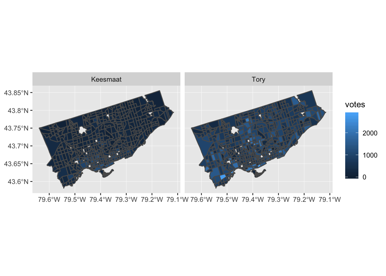
Now that we have votes aggregated by census tract, we can add in many other attributes from the census data. We won’t do that here, since this post is already pretty long. But, we’ll end with a plot to show how easily sf integrates with ggplot2. This is a nice improvement from past workflows, when several steps were required. In the actual code for the retrospective analysis, I added some other plotting techniques, like cutting the response variable (votes) into equally spaced pieces and adding some more refined labels. Here, we’ll just produce a simple plot.
ggplot2::ggplot(data = ct_votes) +
  ggplot2::geom_sf(ggplot2::aes(fill = votes)) +
  ggplot2::facet_wrap(~candidate)