code
- Notifications of relevant new messages.
- A process for keeping track of important and unanswered messages.
- Automatic archiving with excellent search capabilities.
- Portability and easy access.
- Mark photos with the check-mark tag
- Run the image2web script
- Past the clipboard to Blapp
- Publish the weblog
expand.grid
Here’s a simple trick for creating experimental designs in R: use the function expand.grid.
A simple example is:
  treatments <- LETTERS[1:4]
  levels <- 1:3
  experiment <- data.frame(expand.grid(treatment=treatments, level=levels))
which produces:
   treatment level
1          A     1
2          B     1
3          C     1
4          D     1
5          A     2
6          B     2
7          C     2
8          D     2
9          A     3
10         B     3
11         C     3
12         D     3
Now, if you want to randomize your experimental treatments, try:
experiment[sample(dim(experiment)[1]), ]
sample randomly chooses numbers from a vector the same length as the experiment data frame without replacement. The square brackets then use this random sample to subsample from the experiment data frame.
Heart of the Matter
CBC’s Ideas has been running a series of shows on heart disease called “Heart of the Matter”. Episode 2 is particularly interesting from a statistical perspective, as the episode discusses several difficulties with the analysis of drug efficacy. Some highlights include:
Effect sizes Some of the best cited studies for the use of drugs to treat heart disease show a statistically significant effect of only a few percentage points improvement. Contrast this with a dramatic, vastly superior improvement from diet alone.
Response variables The focus of many drug studies has been on the reduction of cholesterol, rather than reductions in heart disease. Diet studies, for example, have shown dramatic improvements in reducing heart attacks while having no effect on cholesterol levels. Conversely, drug studies that show a reduction in cholesterol show no change in mortality rates.
Blocking of data Separate analyses of drug efficacy on female or elderly patients tend to show that drug therapy increases overall mortality. Lumping these data in with the traditional middle-aged male patients removes this effect and, instead, shows a significant decrease in heart disease with drug use.
The point here isn’t to make a comment on the influence of drug companies on medical research. Rather, such statistical concerns are common to all research disciplines. The primary concern of such analyses should be: what is the magnitude of the effect of a specific treatment on my variable of interest? The studies discussed in the Ideas program suggest that much effort has been devoted to detecting significant effects of drugs on surrogate response variables regardless of the size of the effect.
Plantae resurrected
Some technical issues coupled with my road-trip-without-a-laptop conspired to keep Plantae from working correctly. I’ve repaired the damage and isolated Plantae from such problems in the future. My apologies for the downtime.
Analysis of Count Data
When response variables are composed of counts, the standard statistical methods that rely on the normal distribution are no longer applicable. Count data are comprised of positive integers and, often, many zeros. For such data, we need statistics based on Poisson or binomial distributions. I’ve spent the past few weeks analysing counts from hundreds of transects and, as is typical, a particular challenge was determining the appropriate packages to use for R. Here’s what I’ve found so far.
The first step is to get an idea of the dispersion of data points:
Means <- tapply(y, list(x1, x2), mean)
Vars <- tapply(y, list(x1, x2), var)
plot(Means, Vars, xlab="Means", ylab="Variances")
abline(a=0, b=1)
For the Poisson distribution, the mean is equal to the variance. So, we expect the points to lie along the solid line added to the plot. If the points are overdispersed, a negative binomial link function may be more appropriate. The pscl library provides a function to test this:
library(pscl)
model.nb <- glm.nb(y ~ x, data=data)
odTest(model.nb)
summary(model.nb)
If the odTest function rejects the null model, then the data are overdispersed relative to a Poisson distribution. One particularly useful function is glmmPQL from the MASS library. This function allows for random intercepts and combined with the negative.binomial function of the same library, you can fit a negative binomial GLMM:
model.glmm.nb <- glmmPQL(y ~ x1 + x2,
                         random= ~ 1|transect, data=data,
                         family=negative.binomial(model.nb$theta))
In this case, I use the Θ estimated from the glm.nb function in the negative.binomial call. Also useful are the zeroinfl function of the pscl library for fitting zero-inflated Poisson or negative binomial models and the geeglm function of geepack for fitting generalized estimating equations for repeated measures. Finally, fitdistr from MASS allows for estimating the parameters of different distributions from empirical data.
Desktop Manager
I’m convinced that no computer display is large enough. What we need are strategies to better manage our computer workspace and application windows. Exposé and tabbed browsing are great features, but what I really want is the equivalent of a file folder. You put all of the relevant documents in a folder and then put it aside for when you need it. Once you’re ready, you open up the folder and are ready to go.
A feature that comes close to this is virtual desktops. I became enamoured with these while running KDE and have found them again for OS X with Desktop Manager. The idea is to create workspaces associated with specific tasks as a virtual desktop. You can then switch between these desktops as you move from one project to the next. So, for each of the projects I am currently working on, I’ve created a desktop with each application’s windows in the appropriate place. For a consulting project, I likely have Aquamacs running an R simulation with a terminal window open for updating my subversion repository. A project in the writing stage requires TeXShop and BibDesk, while a web-design project needs TextMate and Camino. Each of these workspaces is independent and I can quickly switch to them when needed. Since the applications are running with their windows in the appropriate place, I can quickly get back to work on the project at hand.
Application windows can be split across desktops and specific windows can be present across all desktops. I’ve also found it useful to have one desktop for communication (email, messaging, etc.) and another that has no windows open at all.
Managing project files
As I accumulate projects (both new and completed), the maintenance and storage of the project files becomes increasingly important. There are two important goals for a file structure: find things quickly and don’t lose anything. My current strategy is as follows:
Every project has a consistent folder structure:
|-- analysis
|-- data
|-- db
|-- doc
|-- fig
`-- utils
analysis holds the R source files of the analysis. These, typically, are experiments and snippets of code. The main analyses are in the doc directory.
data contains data files. Generally, these are csv files from clients.
db is for sql dumps of databases and sqlite files. I prefer working with databases over flat text files or Excel spreadsheets. These files are kept in the data folder and converted to sql databases for analyses.
doc holds the analysis and writeup as a Sweave file. This combines R and LaTeX to create a complete document from one source file.
fig is for diagrams and plots. Many of these are generated when processing the Sweave file, but some are constructed from other sources.
utils holds scripts and binaries that are required to run the analysis.
This entire directory structure is maintained with Subversion, so I have a record of changes and can access the project files from any networked computer.
Finally, once a project is complete, I archive the project and construct a sha checksum of the zip file.
openssl dgst -sha1 -out checksums.txt archive.zip
This checksum allows me to verify that the archive remains stable over time. Coupled with a good backup routine, this should keep the project files safe.
This may seem elaborate, but data and their analyses are too important to be left scattered around a laptop’s hard drive.
One other approach I’ve considered is using the R package structure to maintain projects. This is a useful guide, but the process seems too involved for my purposes.
Sun grid
Sun’s new Grid Compute Utility could be a great resource. As I described in an earlier post, running simulations can be a challenge with limited computer resources. Rather than waiting hours for my computers to work through thousands of iterations, I could pay Sun $1, which would likely be sufficient for the scale of my work. This would be well worth the investment! I spend a single dollar and quickly get the results I need for my research or clients.
Apparently, the American government has classified the Sun Grid as a weapon, so we can’t access it here in Canada, yet. I’m sure this will change shortly.
Automator, Transmit, and Backup
The Strongspace weblog has a useful post about using Transmit and Automator to make backups. One challenge with this approach is backing up files scattered throughout your home folder. The solution is the “Follow symbolic links” option when mirroring. I created a backup folder and populated it with aliases to the files I’m interested in backing up. Mirroring this folder to Strongspace copies the files to the server. The other option is to use the “Skip files with specified names” feature, but this rapidly filled up for me.
Remote data analysis
My six-year old laptop is incredibly slow, particularly when analysing data. Unfortunately, analysing data is my job, so this represents a problem. We have a new and fast desktop at home, but I can’t monopolise its use and it would negate the benefits of mobility.
Fortunately, with the help of Emacs and ESS there is a solution. I write my R code on the laptop and evaluate the code on the desktop, which sends the responses and plots back to the laptop. I can do this anywhere I have network access for the laptop and the results are quite quick.
There are a few tricks to the setup, especially if you want the plots sent back to the laptop’s screen, so I’ll document the necessary steps here.
First, you need to enable X11 forwarding on both the desktop and laptop computers (see the Apple Technote). Then start up X11 on the laptop.
Now, on the laptop, start up Emacs, open a file with R code and ssh to the desktop:
opt-x ssh -Y desktopip
Now, run R in the ssh buffer and link it to the R-code buffer
R opt-x ess-remote
That should do it. Now I have the speed of the desktop and the benefits of a laptop.
Rails, sqlite3, and id=0
I’ve spent the last few days struggling with a problem with Plantae’s rails code. I was certain that code like this should work:
class ContentController < ApplicationController
  def new
    @plant = Plant.new(params[:plant])
    if request.post? and @plant.save
      redirect_to :action => 'show', :id => @plant.id
    else
       ...
    end
  end

  def show
    @plant = Plant.find(params[:id])
  end
  ...
end
These statements should create a new plant and then redirect to the show method which sends the newly created plant to the view.
The problem was that rails insisted on asking sqlite3 for the plant with id=0, which cannot exist.
After a post to the rails mailing list and some thorough diagnostics I discovered this and realized I needed swig.
So, if anyone else has this problem:
sudo port install swig
sudo gem install sqlite3-ruby
is the solution.
Taxonomy release
Plantae now supports the addition and updating of species names and families. A rather important first step. Now onto adding character data to make the site actually useful.
Breakpoint regression
In my investigations of ovule fates, I’ve needed to estimate regression parameters from discontinuous functions. A general term for such estimates is breakpoint regression. OFStatisticalEstimates.pdf demonstrates an approach using R for such estimates in the context of seed-ovule ratios. The code includes a mechanism for generating seed-ovule data that illustrate the types of functions that need to be considered.
Managing Email
I recently lost control of my email. The combination of mailing lists, alerts, table of content notifications, and actual email from friends and colleagues was reaching a few hundred emails a day. The insanity had to stop! Here’s how I regained control.
Goals
Before describing my solution, let’s consider what a good email system should provide?
Strategy
I implemented my strategy as I switched to a Gmail account, which required that I catalogue and cancel all of my email subscriptions. Rather than re-subscribing to these, I redirected as many as possible to NetNewsWire. Many journals now provide feeds for their table of content alerts (e.g., Nature) and most of the important newsgroups are available through Gmane. The advantage of news feeds over email alerts is that I can easily group the alerts and choose when to refresh the subscriptions. Typically, I refresh my feed subscriptions in the morning as I caffeinate. I can simply flag important threads or articles for followup later if necessary and my Inbox is no longer cluttered.
Switching to Gmail also immediately solved several other issues with email. First, I no longer worry about storing and archiving email. All of it stays on Google’s servers. Second, this also solves the problem of deciding which messages to keep. Previously, for every new message I had to decide whether to delete it forever or store a copy. Although this only takes a few seconds for each message, when you receive hundreds of messages this can add up. Now, I don’t worry about it. I know that with the combination of Gmail’s search capabilities and my Mac’s Spotlight technology, I can find messages almost instantly. Third, Gmail is available from any webbrowser – now, so is my email.
That’s great so far, but I still have a variety of unfiltered email and I want to only be alerted to important or relevant messages. This is where Mail.app’s smart mailboxes and rules become important. The most important rule is that a message from someone who is not in my Address Book is immediately redirected out of my Inbox. I’ve also implemented a variety of aliases that allows easy filtering of email from my Inbox. All of these filtered messages are gathered together in a folder which I, generally, peruse once a day.
Now I’m left with an Inbox containing only messages from people that I know. As new mail arrives, any mail that survives my filters is sent to Growl and an unobtrusive notification apprises me of the sender and subject. I can then choose to ignore the message if I’m busy or switch to Mail and read the message if it appears to be important.
As I process my messages, I implement the GTD workflow: if responding takes less than two minutes, I respond; otherwise, the message is flagged for follow-up. Finally, I have two smart mailboxes: flagged messages; and messages received today. Since I’ve asked Mail to group messages by thread, today’s messages also pull in all of my previous correspondence on the subject. Messages in these two mailboxes are what appear in my main message window. When I switch to Mail all I see are flagged, and therefore important, messages and current conversations.
This all may seem elaborate, but I find it works well.
iTunes remote control
The current setup at home is that I’ve added all of our music (several thousand songs) to our Mac Mini and then send it through AirTunes to the home stereo. The complication is that the stereo and computer are at opposite ends of the house. Ideally, I can use my iBook to control the Mac Mini without needing to walk down the hall, but how?
One solution is to use VNC, which allows complete control of the Mac Mini. Essentially, the iBook becomes a remote keyboard, mouse, and display. However, I generally only want to either toggle iTunes between play and pause or skip to the next track. Loading up a VNC client and interacting with iTunes directly seems excessive in this case.
An alternate approach I have taken relies on a Terminal session and osascript. The first step is to log into the Mac Mini:
$ ssh Nexus.local. -p 22
Then I can toggle between play and pause with:
$ osascript -e 'tell application "itunes" to playpause'
or skip the current track with:
$ osascript -e 'tell application "itunes" to nexttrack'
I keep the Terminal session active and have added the osascript commands to Textpander so that I can quickly control iTunes remotely.
Combining pdf files
Recently, I needed to combine several pdf files into one. The The Tao of Mac has a discussion of how to do this and I’m posting the code I used here so that I can find it again later.
gs -dNOPAUSE -dBATCH -sDEVICE=pdfwrite -sOutputFile=out.pdf -c save pop -f *.pdf
Running this from a directory containing only the pdfs to be combined produces out.pdf.
Vector assignment in R
As I use R for data analysis and simulations, I become more comfortable and proficient with the R/S syntax and style of programming. One important insight is the use of vector assignments in simulations. I have often read that using such assignments is the preferred method, but until recently I had not realised the importance of this statement. To illustrate the use of vector assignments and their advantages, consider two models of the style illustrated below:
Model 1:
 value1List <- seq(1:10)
 value2Function <- function (value1) {
     ifelse(value1 < constant1, constant2, constant1)
 }
 tableDimension <- length(value1List)
 outputTable <- NULL
 outputTable <- data.frame(value1=numeric(tableDimension),
 value2=numeric(tableDimension))
 n <- 1
 for (value1 in value1List) {
     outputTable[n, ] <- c(value1, value2Function(value1))
     n <- n + 1
 }
Model 2:
 value1List <- seq(1:10)
 tableDimension <- length(value1List)
 outputTable <- NULL
 outputTable$value1 <- rep(value1List, each=
     tableDimension / (length(value1List)))
 outputTable <- as.data.frame(outputTable)
 outputTable$value2 <- ifelse(value1 < constant1, constant2, constant1)
Model 1 is how I originally approached R programming. It begins with declaration of a sequence for value1 and a function declaration to calculate value2 from each value1. I then declare a table to capture the output and fill it with zero values. The main loop of the program consists of replacing the rows of the output table with each value of value1 and the calculated value2. I use the variable n to keep track of the next row in the table. The function rbind() could also be used to generate the table, but it’s use for large datasets is quite inefficient.
Model 2 takes the approach of constructing each column of the output table in sequence. It begins by repeating the values of the value1List and then creates the value2 column through a vector assignment. No control structures or function calls are required in Model 2.
How is this important? Model 1 seems intuitive (at least to me) while the syntax of Model 2 is opaque at first glance. However, consider this figure:
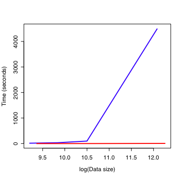
On the x-axis is the number of data points in the output table on a log scale. The y-axis shows how long the model takes to calculate these values. Model 1 is the blue line. Model 2 is the red line. This illustrates two important points: * Model 1 is always slower than Model 2. * As the size of the dataset increases, Model 2 remains fast while Model 1 rapidly consumes all of the computer resources.
This is why vector assignments should be used when programming with R. Just to be clear, the models described here are simple abstractions of the types of models used to generate this figure.
Image uploads
A particular challenge with maintaining a weblog is the uploading and resizing of images. The process involves choosing the correct images, creating large & thumbnail sized versions, uploading these images to the webserver, and posting the appropriate code into the weblog post. In the spirit of my last few posts, image2web is an applescript I use to automate this process:
  --user-specific variables
  property theAlbum : "Marked"
      --contains the images to be uploaded
  property theBasePath : "the:path:to:the:local:images:" as alias
      --the local path to the weblog
  property tagBaseUrl : "[www.your.website.org/path/to//...](http://www.your.website.org/path/to//blog/images/)"
      --the url to the weblog images
  ---declare globals
  property htmlText : ""
      --stores the image tags & is copied to the clipboard

  tell application "Finder"
      set theList to name of every folder of theBasePath
  end tell

  --choose which weblog category the images belong to
  set theCategoryList to choose from list theList
      with prompt "Choose the post's category:"
  set theCategory to first item of theCategoryList

  tell application "Finder"
      set theCategoryFolder to folder theCategory of theBasePath
  end tell

  --I use a smart album that collects photos with the checkmark tag
  tell application "iPhoto"
      activate
      select album theAlbum --so we can see which images are involved
      set theImages to every photo of album theAlbum --collect the images
      repeat with thisImage in theImages
          set thisImage to get image path of thisImage
          my processImage(thisImage, theCategoryFolder)
      --resize & generate the thumbnail
      set theResult to the result --avoid declaring more globals
      set thePhotoName to item 1 of theResult
      set theMainImagePath to item 2 of theResult
      set theThumbnailImagePath to item 3 of theResult
      my uploadImage(theMainImagePath, theThumbnailImagePath) --upload the image
      my makeTag(theCategory, thePhotoName) --create the appropriate html
      end repeat
      set the clipboard to htmlText --pass the html code to the clipboard
  end tell

  on processImage(thisImage, theCategoryFolder)

      set theResult to display dialog "Enter the name for " & thisImage & ":" default answer ""
      set thePhotoName to text returned of theResult

      tell application "Finder"
          set theDestinationPath to POSIX path of (theCategoryFolder as string)
          set theMainImagePath to (theDestinationPath & thePhotoName & ".jpg")
          set theThumbnailImagePath to (theDestinationPath & thePhotoName & "-thumb.jpg")
          do shell script "/usr/local/bin/convert -resize 640x480 +profile \" * \" " & "\""
      & thisImage & "\"" & " " & theMainImagePath
      ---use extra quotes to protect against spaces in path names
          do shell script "/usr/local/bin/convert -resize 240x240 +profile \" * \" " & "\""
      & thisImage & "\"" & " " & theThumbnailImagePath
      end tell
      return {thePhotoName, theMainImagePath, theThumbnailImagePath}

  end processImage

  on uploadImage(theMainImagePath, theThumbnailImagePath)

      set theMainImage to POSIX file theMainImagePath
      set theThumbnailImage to POSIX file theThumbnailImagePath

      tell application "Transmit"
          open theMainImage
          open theThumbnailImage
      end tell

  end uploadImage

  on makeTag(theCategory, thePhotoName)
	set htmlText to htmlText & ""
      --show the thumbnail & link to the full-size image
  end makeTag
The workflow is as follows:
This script requires both ImageMagick and Transmit and is inspired by a script from waferbaby.
Quirks & Quarks
Quirks & Quarks is the CBC’s excellent science program. I usually download the mp3 archives of the show on the weekends and listen while I walk Ceiligh.
Of course, loading up the Quirks & Quarks webpage, finding the archives, downloading the mp3s, and adding them to iTunes takes at least a few minutes. Computers are much better and handling such tedium.
Inspired by the success (for me) of the apod script, quirks.pl is a perl script that downloads the current Quirks & Quarks episode to the Desktop. runQuirks.scpt is an applescript that further simplifies the process by adding the downloads to iTunes and trashing the redundant downloads. I’ve set iCal to invoke runQuirks.scpt in the middle of the night, so now Quirks & Quarks is on my iPod and ready to go Sunday morning.
Note that runQuirks.scpt expects quirks.pl to be in “~/Library/Scripts/quirks/”.
Astronomy pictures on the Desktop
The “Astronomy Picture of the Day” is a source of fantastic images. To take advantage of this resource, I went looking for a way to automatically set the current image as my Desktop background. A quick Google search turned up a perl script at www.haroldbakker.com. Although this was a great start, I wasn’t completely happy with the implementation of this script and decided to write my own.
The apod.pl script is written in perl and both sets the Desktop background and copies a description of the image to the Desktop as an html file. You can add the script to your Script menu and run it as appropriate. Even better, download the runApod.scpt applescript and have iCal set the Desktop at a convenient time. I’ve set up my computer to run the perl script early each morning so that I have a new Desktop background each day. Note that runApod.scpt expects apod.pl to be in “~/Library/Scripts/apod/”.
JSTOR import script
I’ve written a script that imports a JSTOR citation page into BibDesk. To use the script, I suggest adding it to your script menu. Then, with the JSTOR citation page as the active web page in Safari, run the script and the citation will be added to the active BibDesk file. I use the first author’s last name and last two digits of the year as a cite key (e.g. Darwin59), you may want to change this to suit your style.
The script is written in perl and bracketed by two Applescript commands: one to extract the html source from the JSTOR page and the other to add the citation to BibDesk. Unfortunately, JSTOR citation pages contain almost no semantic markup, so I am not convinced that the approach is entirely robust. However, so far it has worked well for me and might be useful to you. Any feedback is welcome.
Download the script. JSTORImport.pl.txt