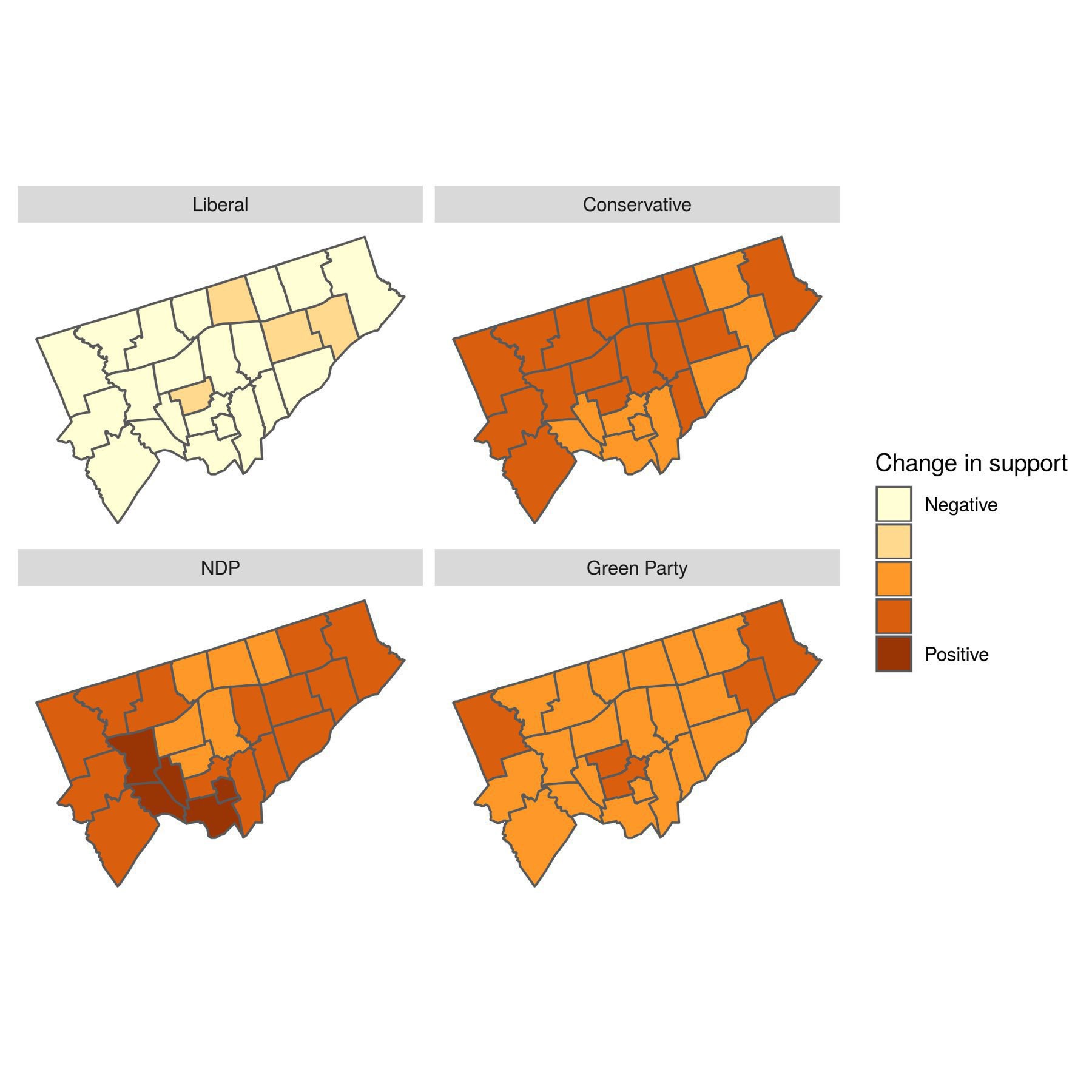
We’ve compared our predictions of the 2019 🇨🇦 election to the actual votes. Overall, we were within 5% with no obvious geographical biases, though we did slightly overestimate support for the NDP at the expense of the Liberals. I think we’re on to something good here!
election
With an agent based model you can explore interesting scenarios. Our latest post models the 🇨🇦 election with another Liberal scandal, new Conservatives climate change policy, or proportional representation. The results are not obvious, showing benefits of non-linear modelling.
Spatial analysis of votes in Toronto
Tuesday, December 4, 2018
This is a “behind the scenes” elaboration of the geospatial analysis in our recent post on evaluating our predictions for the 2018 mayoral election in Toronto. This was my first, serious use of the new sf package for geospatial analysis. I found the package much easier to use than some of my previous workflows for this sort of analysis, especially given its integration with the tidyverse.
We start by downloading the shapefile for voting locations from the City of Toronto’s Open Data portal and reading it with the read_sf function. Then, we pipe it to st_transform to set the appropriate projection for the data. In this case, this isn’t strictly necessary, since the shapefile is already in the right projection. But, I tend to do this for all shapefiles to avoid any oddities later.
download.file("http://opendata.toronto.ca/gcc/voting_location_2018_wgs84.zip",
                destfile = "data-raw/voting_location_2018_wgs84.zip", quiet = TRUE)
unzip("data-raw/voting_location_2018_wgs84.zip", exdir="data-raw/voting_location_2018_wgs84")
toronto_locations <- sf::read_sf("data-raw/voting_location_2018_wgs84",
                                 layer = "VOTING_LOCATION_2018_WGS84") %>%
  sf::st_transform(crs = "+init=epsg:4326")
toronto_locations
## Simple feature collection with 1700 features and 13 fields
## geometry type:  POINT
## dimension:      XY
## bbox:           xmin: -79.61937 ymin: 43.59062 xmax: -79.12531 ymax: 43.83052
## epsg (SRID):    4326
## proj4string:    +proj=longlat +datum=WGS84 +no_defs
## # A tibble: 1,700 x 14
##    POINT_ID FEAT_CD FEAT_C_DSC PT_SHRT_CD PT_LNG_CD POINT_NAME VOTER_CNT
##       <dbl> <chr>   <chr>      <chr>      <chr>     <chr>          <int>
##  1    10190 P       Primary    056        10056     <na>              37
##  2    10064 P       Primary    060        10060     <na>             532
##  3    10999 S       Secondary  058        10058     Malibu           661
##  4    11342 P       Primary    052        10052     <na>            1914
##  5    10640 P       Primary    047        10047     The Summit       956
##  6    10487 S       Secondary  061        04061     White Eag…        51
##  7    11004 P       Primary    063        04063     Holy Fami…      1510
##  8    11357 P       Primary    024        11024     Rosedale …      1697
##  9    12044 P       Primary    018        05018     Weston Pu…      1695
## 10    11402 S       Secondary  066        04066     Elm Grove…        93
## # ... with 1,690 more rows, and 7 more variables: OBJECTID <dbl>,
## #   ADD_FULL <chr>, X <dbl>, Y <dbl>, LONGITUDE <dbl>, LATITUDE <dbl>,
## #   geometry <point>
The file has 1700 rows of data across 14 columns. The first 13 columns are data within the original shapefile. The last column is a list column that is added by sf and contains the geometry of the location. This specific design feature is what makes an sf object work really well with the rest of the tidyverse: the geographical details are just a column in the data frame. This makes the data much easier to work with than in other approaches, where the data is contained within an [@data](https://micro.blog/data) slot of an object.
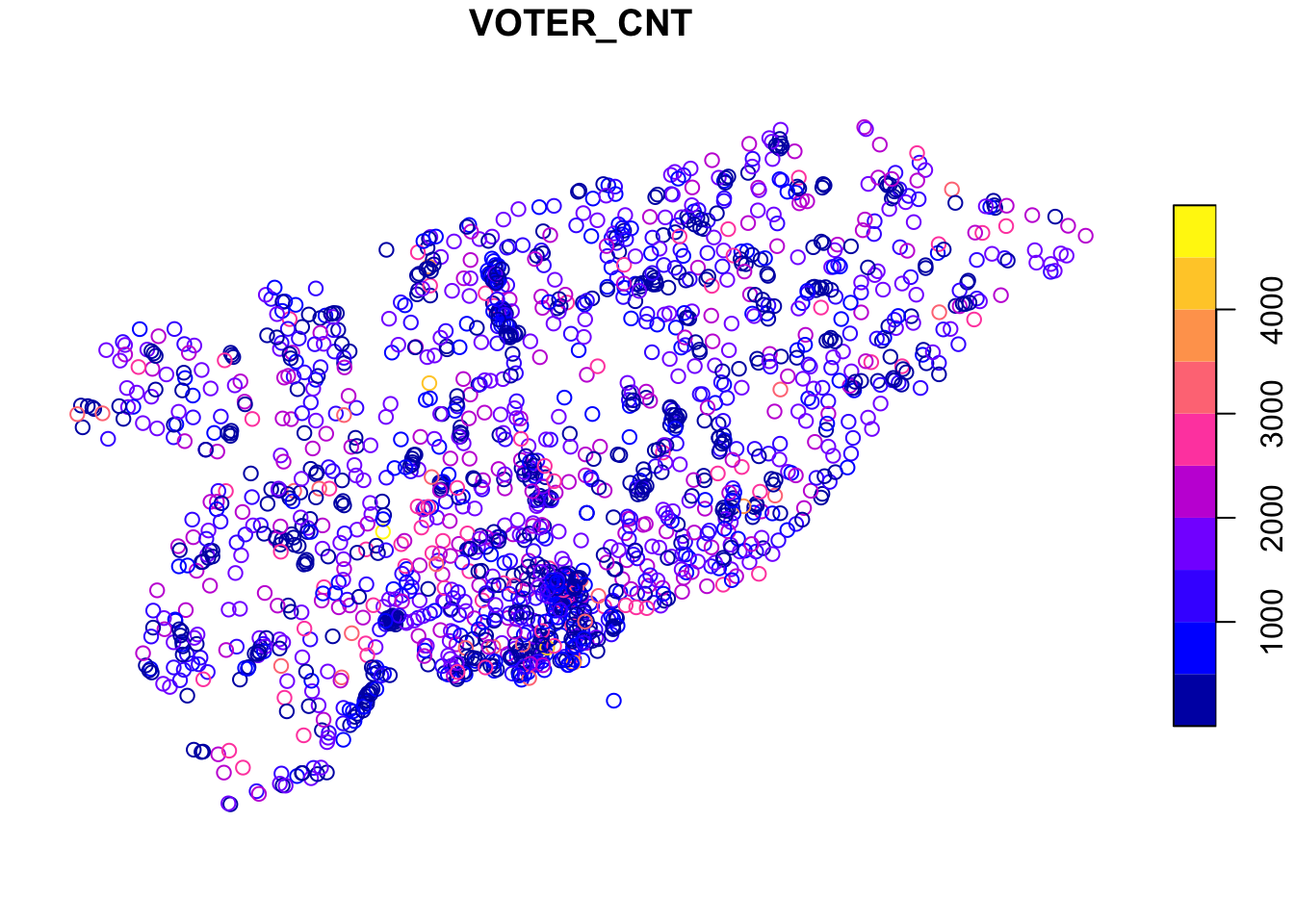
Plotting the data is straightforward, since sf objects have a plot function. Here’s an example where we plot the number of voters (VOTER_CNT) at each location. If you squint just right, you can see the general outline of Toronto in these points.
What we want to do next is use the voting location data to aggregate the votes cast at each location into census tracts. This then allows us to associate census characteristics (like age and income) with the pattern of votes and develop our statistical relationships for predicting voter behaviour.
We’ll split this into several steps. The first is downloading and reading the census tract shapefile.
download.file("http://www12.statcan.gc.ca/census-recensement/2011/geo/bound-limit/files-fichiers/gct_000b11a_e.zip",
                destfile = "data-raw/gct_000b11a_e.zip", quiet = TRUE)
unzip("data-raw/gct_000b11a_e.zip", exdir="data-raw/gct")
census_tracts <- sf::read_sf("data-raw/gct", layer = "gct_000b11a_e") %>%
  sf::st_transform(crs = "+init=epsg:4326")
Now that we have it, all we really want are the census tracts in Toronto (the shapefile includes census tracts across Canada). We achieve this by intersecting the Toronto voting locations with the census tracts using standard R subsetting notation.
to_census_tracts <- census_tracts[toronto_locations,]
And, we can plot it to see how well the intersection worked. This time we’ll plot the CTUID, which is the unique identifier for each census tract. This doesn’t mean anything in this context, but adds some nice colour to the plot.
plot(to_census_tracts["CTUID"])
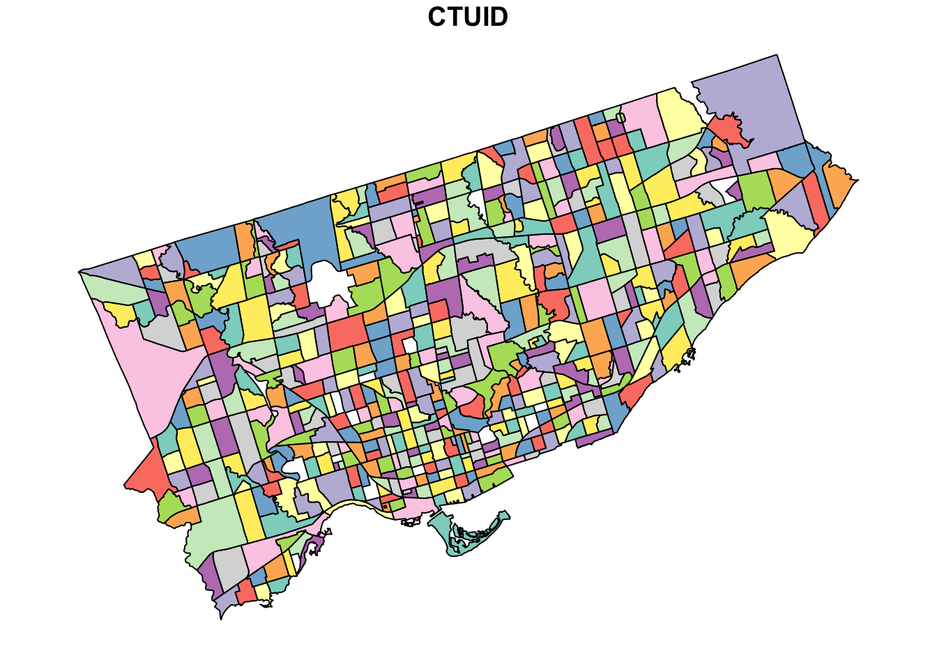
Now you can really see the shape of Toronto, as well as the size of each census tract.
Next we need to manipulate the voting data to get votes received by major candidates in the 2018 election. We take these data from the toVotes package and arbitrarily set the threshold for major candidates to receiving at least 100,000 votes. This yields our two main candidates: John Tory and Jennifer Keesmaat.
major_candidates <- toVotes %>%
  dplyr::filter(year == 2018) %>%
  dplyr::group_by(candidate) %>%
  dplyr::summarise(votes = sum(votes)) %>%
  dplyr::filter(votes > 100000) %>%
  dplyr::select(candidate)
major_candidates
## # A tibble: 2 x 1
##   candidate
##   <chr>
## 1 Keesmaat Jennifer
## 2 Tory John
Given our goal of aggregating the votes received by each candidate into census tracts, we need a data frame that has each candidate in a separate column. We start by joining the major candidates table to the votes table. In this case, we also filter the votes to 2018, since John Tory has been a candidate in more than one election. Then we use the tidyr package to convert the table from long (with one candidate column) to wide (with a column for each candidate).
spread_votes <- toVotes %>%
  tibble::as.tibble() %>%
  dplyr::filter(year == 2018) %>%
  dplyr::right_join(major_candidates) %>%
  dplyr::select(-type, -year) %>%
  tidyr::spread(candidate, votes)
spread_votes
## # A tibble: 1,800 x 4
##     ward  area `Keesmaat Jennifer` `Tory John`
##    <int> <int>               <dbl>       <dbl>
##  1     1     1                  66         301
##  2     1     2                  72         376
##  3     1     3                  40         255
##  4     1     4                  24         161
##  5     1     5                  51         211
##  6     1     6                  74         372
##  7     1     7                  70         378
##  8     1     8                  10          77
##  9     1     9                  11          82
## 10     1    10                  12          76
## # ... with 1,790 more rows
Our last step before finally aggregating to census tracts is to join the spread_votes table with the toronto_locations data. This requires pulling the ward and area identifiers from the PT_LNG_CD column of the toronto_locations data frame which we do with some stringr functions. While we’re at it, we also update the candidate names to just surnames.
to_geo_votes <- toronto_locations %>%
  dplyr::mutate(ward = as.integer(stringr::str_sub(PT_LNG_CD, 1, 2)),
                area = as.integer(stringr::str_sub(PT_LNG_CD, -3, -1))) %>%
  dplyr::left_join(spread_votes) %>%
  dplyr::select(`Keesmaat Jennifer`, `Tory John`) %>%
  dplyr::rename(Keesmaat = `Keesmaat Jennifer`, Tory = `Tory John`)
to_geo_votes
## Simple feature collection with 1700 features and 2 fields
## geometry type:  POINT
## dimension:      XY
## bbox:           xmin: -79.61937 ymin: 43.59062 xmax: -79.12531 ymax: 43.83052
## epsg (SRID):    4326
## proj4string:    +proj=longlat +datum=WGS84 +no_defs
## # A tibble: 1,700 x 3
##    Keesmaat  Tory             geometry
##       <dbl> <dbl>          <point>
##  1       55   101 (-79.40225 43.63641)
##  2       43    53  (-79.3985 43.63736)
##  3       61    89 (-79.40028 43.63664)
##  4      296   348 (-79.39922 43.63928)
##  5      151   204 (-79.40401 43.64293)
##  6        2    11 (-79.43941 43.63712)
##  7      161   174 (-79.43511 43.63869)
##  8      221   605  (-79.38188 43.6776)
##  9       68   213 (-79.52078 43.70176)
## 10        4    14 (-79.43094 43.64027)
## # ... with 1,690 more rows
Okay, we’re finally there. We have our census tract data in to_census_tracts and our voting data in to_geo_votes. We want to aggregate the votes into each census tract by summing the votes at each voting location within each census tract. We use the aggregate function for this.
ct_votes_wide <- aggregate(x = to_geo_votes,
                           by = to_census_tracts,
                           FUN = sum)
ct_votes_wide
## Simple feature collection with 522 features and 2 fields
## geometry type:  MULTIPOLYGON
## dimension:      XY
## bbox:           xmin: -79.6393 ymin: 43.58107 xmax: -79.11547 ymax: 43.85539
## epsg (SRID):    4326
## proj4string:    +proj=longlat +datum=WGS84 +no_defs
## First 10 features:
##    Keesmaat Tory                       geometry
## 1       407  459 MULTIPOLYGON (((-79.39659 4...
## 2      1103 2400 MULTIPOLYGON (((-79.38782 4...
## 3       403 1117 MULTIPOLYGON (((-79.27941 4...
## 4        96  570 MULTIPOLYGON (((-79.28156 4...
## 5       169  682 MULTIPOLYGON (((-79.49104 4...
## 6       121  450 MULTIPOLYGON (((-79.54422 4...
## 7        42   95 MULTIPOLYGON (((-79.45379 4...
## 8       412  512 MULTIPOLYGON (((-79.33895 4...
## 9        83  132 MULTIPOLYGON (((-79.35427 4...
## 10       92  629 MULTIPOLYGON (((-79.44554 4...]
As a last step, to tidy up, we now convert the wide table with a column for each candidate into a long table that has just one candidate column containing the name of the candidate.
ct_votes <- tidyr::gather(ct_votes_wide, candidate, votes, -geometry)
ct_votes
## Simple feature collection with 1044 features and 2 fields
## geometry type:  MULTIPOLYGON
## dimension:      XY
## bbox:           xmin: -79.6393 ymin: 43.58107 xmax: -79.11547 ymax: 43.85539
## epsg (SRID):    4326
## proj4string:    +proj=longlat +datum=WGS84 +no_defs
## First 10 features:
##    candidate votes                       geometry
## 1   Keesmaat   407 MULTIPOLYGON (((-79.39659 4...
## 2   Keesmaat  1103 MULTIPOLYGON (((-79.38782 4...
## 3   Keesmaat   403 MULTIPOLYGON (((-79.27941 4...
## 4   Keesmaat    96 MULTIPOLYGON (((-79.28156 4...
## 5   Keesmaat   169 MULTIPOLYGON (((-79.49104 4...
## 6   Keesmaat   121 MULTIPOLYGON (((-79.54422 4...
## 7   Keesmaat    42 MULTIPOLYGON (((-79.45379 4...
## 8   Keesmaat   412 MULTIPOLYGON (((-79.33895 4...
## 9   Keesmaat    83 MULTIPOLYGON (((-79.35427 4...
## 10  Keesmaat    92 MULTIPOLYGON (((-79.44554 4...
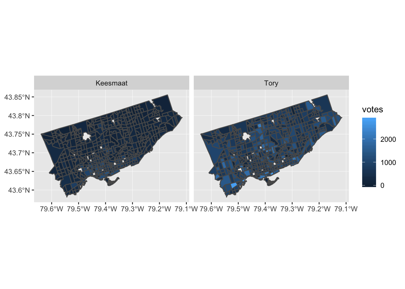
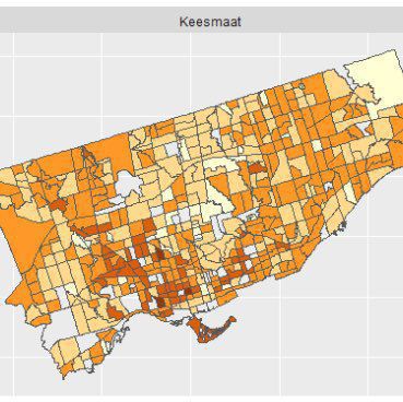
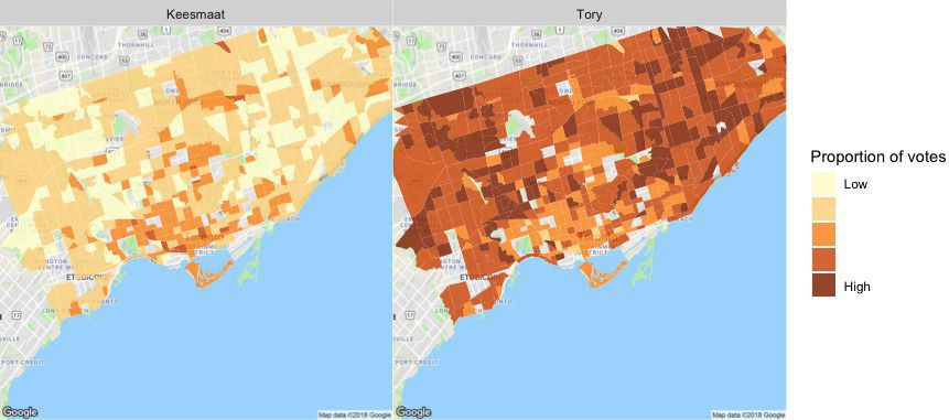
Now that we have votes aggregated by census tract, we can add in many other attributes from the census data. We won’t do that here, since this post is already pretty long. But, we’ll end with a plot to show how easily sf integrates with ggplot2. This is a nice improvement from past workflows, when several steps were required. In the actual code for the retrospective analysis, I added some other plotting techniques, like cutting the response variable (votes) into equally spaced pieces and adding some more refined labels. Here, we’ll just produce a simple plot.
ggplot2::ggplot(data = ct_votes) +
  ggplot2::geom_sf(ggplot2::aes(fill = votes)) +
  ggplot2::facet_wrap(~candidate)
Our predictions for the recent election in Toronto held up well. We were within 6%, on average, with a slight bias towards overestimating Keesmaat’s support. Now we’ll add more demographic richness to our agents and reduce the geographical distribution of errors www.psephoanalytics.ca/2018/11/r…
We’ve completely retooled our approach to predicting elections to use an agent-based model. Looking forward to comparing our predictions to the actual results tonight for the Toronto election!
Fixing a hack finds a better solution
Sunday, September 2, 2018
In my Elections Ontario official results post, I had to use an ugly hack to match Electoral District names and numbers by extracting data from a drop down list on the Find My Electoral District website. Although it was mildly clever, like any hack, I shouldn’t have relied on this one for long, as proven by Elections Ontario shutting down the website.
So, a more robust solution was required, which led to using one of Election Ontario’s shapefiles. The shapefile contains the data we need, it’s just in a tricky format to deal with. But, the sf package makes this mostly straightforward.
We start by downloading and importing the Elections Ontario shape file. Then, since we’re only interested in the City of Toronto boundaries, we download the city’s shapefile too and intersect it with the provincial one to get a subset:
download.file("[www.elections.on.ca/content/d...](https://www.elections.on.ca/content/dam/NGW/sitecontent/2016/preo/shapefiles/Polling%20Division%20Shapefile%20-%202014%20General%20Election.zip)",
              destfile = "data-raw/Polling%20Division%20Shapefile%20-%202014%20General%20Election.zip")
unzip("data-raw/Polling%20Division%20Shapefile%20-%202014%20General%20Election.zip",
      exdir = "data-raw/Polling%20Division%20Shapefile%20-%202014%20General%20Election")
prov_geo <- sf::st_read(“data-raw/Polling%20Division%20Shapefile%20-%202014%20General%20Election”,
layer = “PDs_Ontario”) %>%
sf::st_transform(crs = “+init=epsg:4326”)
download.file("opendata.toronto.ca/gcc/votin…",
destfile = “data-raw/voting_location_2014_wgs84.zip”)
unzip(“data-raw/voting_location_2014_wgs84.zip”, exdir=“data-raw/voting_location_2014_wgs84”)
toronto_wards <- sf::st_read(“data-raw/voting_location_2014_wgs84”, layer = “VOTING_LOCATION_2014_WGS84”) %>%
sf::st_transform(crs = “+init=epsg:4326”)
to_prov_geo <- prov_geo %>%
sf::st_intersection(toronto_wards)
Now we just need to extract a couple of columns from the data frame associated with the shapefile. Then we process the values a bit so that they match the format of other data sets. This includes converting them to UTF-8, formatting as title case, and replacing dashes with spaces:
electoral_districts <- to_prov_geo %>%
  dplyr::transmute(electoral_district = as.character(DATA_COMPI),
                   electoral_district_name = stringr::str_to_title(KPI04)) %>%
  dplyr::group_by(electoral_district, electoral_district_name) %>%
  dplyr::count() %>%
  dplyr::ungroup() %>%
  dplyr::mutate(electoral_district_name = stringr::str_replace_all(utf8::as_utf8(electoral_district_name), "\u0097", " ")) %>%
  dplyr::select(electoral_district, electoral_district_name)
electoral_districts
## Simple feature collection with 23 features and 2 fields
## geometry type: MULTIPOINT
## dimension: XY
## bbox: xmin: -79.61919 ymin: 43.59068 xmax: -79.12511 ymax: 43.83057
## epsg (SRID): 4326
## proj4string: +proj=longlat +datum=WGS84 +no_defs
## # A tibble: 23 x 3
## electoral_distri… electoral_distric… geometry
##
## 1 005 Beaches East York (-79.32736 43.69452, -79.32495 43…
## 2 015 Davenport (-79.4605 43.68283, -79.46003 43.…
## 3 016 Don Valley East (-79.35985 43.78844, -79.3595 43.…
## 4 017 Don Valley West (-79.40592 43.75026, -79.40524 43…
## 5 020 Eglinton Lawrence (-79.46787 43.70595, -79.46376 43…
## 6 023 Etobicoke Centre (-79.58697 43.6442, -79.58561 43.…
## 7 024 Etobicoke Lakesho… (-79.56213 43.61001, -79.5594 43.…
## 8 025 Etobicoke North (-79.61919 43.72889, -79.61739 43…
## 9 068 Parkdale High Park (-79.49944 43.66285, -79.4988 43.…
## 10 072 Pickering Scarbor… (-79.18898 43.80374, -79.17927 43…
## # ... with 13 more rows In the end, this is a much more reliable solution, though it seems a bit extreme to use GIS techniques just to get a listing of Electoral District names and numbers.
Elections Ontario official results
Sunday, November 19, 2017
In preparing for some PsephoAnalytics work on the upcoming provincial election, I’ve been wrangling the Elections Ontario data. As provided, the data is really difficult to work with and we’ll walk through some steps to tidy these data for later analysis.
Here’s what the source data looks like:
Screenshot of raw Elections Ontario data
A few problems with this:
- The data is scattered across a hundred different Excel files
- Candidates are in columns with their last name as the header
- Last names are not unique across all Electoral Districts, so can’t be used as a unique identifier
- Electoral District names are in a row, followed by a separate row for each poll within the district
- The party affiliation for each candidate isn’t included in the data
So, we have a fair bit of work to do to get to something more useful. Ideally something like:
## # A tibble: 9 x 5
##   electoral_district  poll candidate   party votes
##                <chr> <chr>     <chr>   <chr> <int>
## 1                  X     1         A Liberal    37
## 2                  X     2         B     NDP    45
## 3                  X     3         C      PC    33
## 4                  Y     1         A Liberal    71
## 5                  Y     2         B     NDP    37
## 6                  Y     3         C      PC    69
## 7                  Z     1         A Liberal    28
## 8                  Z     2         B     NDP    15
## 9                  Z     3         C      PC    34
This is much easier to work with: we have one row for the votes received by each candidate at each poll, along with the Electoral District name and their party affiliation.
Candidate parties
As a first step, we need the party affiliation for each candidate. I didn’t see this information on the Elections Ontario site. So, we’ll pull the data from Wikipedia. The data on this webpage isn’t too bad. We can just use the table xpath selector to pull out the tables and then drop the ones we aren’t interested in.
``` candidate_webpage <- "https://en.wikipedia.org/wiki/Ontario_general_election,_2014#Candidates_by_region" candidate_tables <- "table" # Use an xpath selector to get the drop down list by IDcandidates <- xml2::read_html(candidate_webpage) %>% rvest::html_nodes(candidate_tables) %>% # Pull tables from the wikipedia entry .[13:25] %>% # Drop unecessary tables rvest::html_table(fill = TRUE)
</pre> <p>This gives us a list of 13 data frames, one for each table on the webpage. Now we cycle through each of these and stack them into one data frame. Unfortunately, the tables aren’t consistent in the number of columns. So, the approach is a bit messy and we process each one in a loop.</p> <pre class="r"><code># Setup empty dataframe to store results candidate_parties <- tibble::as_tibble( electoral_district_name = NULL, party = NULL, candidate = NULL ) for(i in seq_along(1:length(candidates))) { # Messy, but works this_table <- candidates[[i]] # The header spans mess up the header row, so renaming names(this_table) <- c(this_table[1,-c(3,4)], "NA", "Incumbent") # Get rid of the blank spacer columns this_table <- this_table[-1, ] # Drop the NA columns by keeping only odd columns this_table <- this_table[,seq(from = 1, to = dim(this_table)[2], by = 2)] this_table %<>% tidyr::gather(party, candidate, -`Electoral District`) %>% dplyr::rename(electoral_district_name = `Electoral District`) %>% dplyr::filter(party != "Incumbent") candidate_parties <- dplyr::bind_rows(candidate_parties, this_table) } candidate_parties</code></pre> <pre># A tibble: 649 x 3
electoral_district_name party candidate
1 Carleton—Mississippi Mills Liberal Rosalyn Stevens
2 Nepean—Carleton Liberal Jack Uppal
3 Ottawa Centre Liberal Yasir Naqvi
4 Ottawa—Orléans Liberal Marie-France Lalonde
5 Ottawa South Liberal John Fraser
6 Ottawa—Vanier Liberal Madeleine Meilleur
7 Ottawa West—Nepean Liberal Bob Chiarelli
8 Carleton—Mississippi Mills PC Jack MacLaren
9 Nepean—Carleton PC Lisa MacLeod
10 Ottawa Centre PC Rob Dekker
# … with 639 more rows
</pre> </div> <div id="electoral-district-names" class="section level2"> <h2>Electoral district names</h2> <p>One issue with pulling party affiliations from Wikipedia is that candidates are organized by Electoral District <em>names</em>. But the voting results are organized by Electoral District <em>number</em>. I couldn’t find an appropriate resource on the Elections Ontario site. Rather, here we pull the names and numbers of the Electoral Districts from the <a href="https://www3.elections.on.ca/internetapp/FYED_Error.aspx?lang=en-ca">Find My Electoral District</a> website. The xpath selector is a bit tricky for this one. The <code>ed_xpath</code> object below actually pulls content from the drop down list that appears when you choose an Electoral District. One nuisance with these data is that Elections Ontario uses <code>--</code> in the Electoral District names, instead of the — used on Wikipedia. We use <code>str_replace_all</code> to fix this below.</p> <pre class="r"><code>ed_webpage <- "https://www3.elections.on.ca/internetapp/FYED_Error.aspx?lang=en-ca" ed_xpath <- "//*[(@id = \"ddlElectoralDistricts\")]" # Use an xpath selector to get the drop down list by ID electoral_districts <- xml2::read_html(ed_webpage) %>% rvest::html_node(xpath = ed_xpath) %>% rvest::html_nodes("option") %>% rvest::html_text() %>% .[-1] %>% # Drop the first item on the list ("Select...") tibble::as.tibble() %>% # Convert to a data frame and split into ID number and name tidyr::separate(value, c("electoral_district", "electoral_district_name"), sep = " ", extra = "merge") %>% # Clean up district names for later matching and presentation dplyr::mutate(electoral_district_name = stringr::str_to_title( stringr::str_replace_all(electoral_district_name, "--", "—"))) electoral_districts</code></pre> <pre># A tibble: 107 x 2
electoral_district electoral_district_name
1 001 Ajax—Pickering
2 002 Algoma—Manitoulin
3 003 Ancaster—Dundas—Flamborough—Westdale
4 004 Barrie
5 005 Beaches—East York
6 006 Bramalea—Gore—Malton
7 007 Brampton—Springdale
8 008 Brampton West
9 009 Brant
10 010 Bruce—Grey—Owen Sound
# … with 97 more rows
</pre> <p>Next, we can join the party affiliations to the Electoral District names to join candidates to parties and district numbers.</p> <pre class="r"><code>candidate_parties %<>% # These three lines are cleaning up hyphens and dashes, seems overly complicated dplyr::mutate(electoral_district_name = stringr::str_replace_all(electoral_district_name, "—\n", "—")) %>% dplyr::mutate(electoral_district_name = stringr::str_replace_all(electoral_district_name, "Chatham-Kent—Essex", "Chatham—Kent—Essex")) %>% dplyr::mutate(electoral_district_name = stringr::str_to_title(electoral_district_name)) %>% dplyr::left_join(electoral_districts) %>% dplyr::filter(!candidate == "") %>% # Since the vote data are identified by last names, we split candidate's names into first and last tidyr::separate(candidate, into = c("first","candidate"), extra = "merge", remove = TRUE) %>% dplyr::select(-first)</code></pre> <pre><code>## Joining, by = "electoral_district_name"</code></pre> <pre class="r"><code>candidate_parties</code></pre> <pre># A tibble: 578 x 4
electoral_district_name party candidate electoral_district
*
1 Carleton—Mississippi Mills Liberal Stevens 013
2 Nepean—Carleton Liberal Uppal 052
3 Ottawa Centre Liberal Naqvi 062
4 Ottawa—Orléans Liberal France Lalonde 063
5 Ottawa South Liberal Fraser 064
6 Ottawa—Vanier Liberal Meilleur 065
7 Ottawa West—Nepean Liberal Chiarelli 066
8 Carleton—Mississippi Mills PC MacLaren 013
9 Nepean—Carleton PC MacLeod 052
10 Ottawa Centre PC Dekker 062
# … with 568 more rows
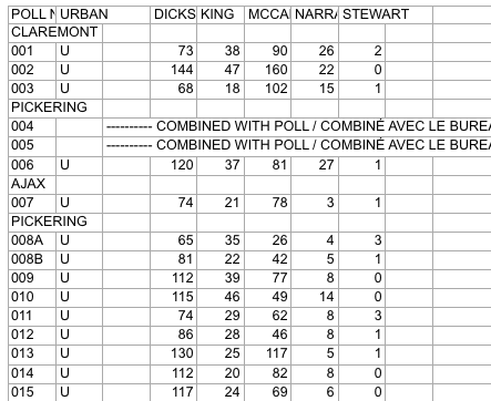
</pre> <p>All that work just to get the name of each candiate for each Electoral District name and number, plus their party affiliation.</p> </div> <div id="votes" class="section level2"> <h2>Votes</h2> <p>Now we can finally get to the actual voting data. These are made available as a collection of Excel files in a compressed folder. To avoid downloading it more than once, we wrap the call in an <code>if</code> statement that first checks to see if we already have the file. We also rename the file to something more manageable.</p> <pre class="r"><code>raw_results_file <- "[www.elections.on.ca/content/d...](http://www.elections.on.ca/content/dam/NGW/sitecontent/2017/results/Poll%20by%20Poll%20Results%20-%20Excel.zip)" zip_file <- "data-raw/Poll%20by%20Poll%20Results%20-%20Excel.zip" if(file.exists(zip_file)) { # Only download the data once # File exists, so nothing to do } else { download.file(raw_results_file, destfile = zip_file) unzip(zip_file, exdir="data-raw") # Extract the data into data-raw file.rename("data-raw/GE Results - 2014 (unconverted)", "data-raw/pollresults") }</code></pre> <pre><code>## NULL</code></pre> <p>Now we need to extract the votes out of 107 Excel files. The combination of <code>purrr</code> and <code>readxl</code> packages is great for this. In case we want to filter to just a few of the files (perhaps to target a range of Electoral Districts), we declare a <code>file_pattern</code>. For now, we just set it to any xls file that ends with three digits preceeded by a “_“.</p> <p>As we read in the Excel files, we clean up lots of blank columns and headers. Then we convert to a long table and drop total and blank rows. Also, rather than try to align the Electoral District name rows with their polls, we use the name of the Excel file to pull out the Electoral District number. Then we join with the <code>electoral_districts</code> table to pull in the Electoral District names.</p> <pre class="r">file_pattern <- “*_[[:digit:]]{3}.xls” # Can use this to filter down to specific files poll_data <- list.files(path = “data-raw/pollresults”, pattern = file_pattern, full.names = TRUE) %>% # Find all files that match the pattern purrr::set_names() %>% purrr::map_df(readxl::read_excel, sheet = 1, col_types = “text”, .id = “file”) %>% # Import each file and merge into a dataframe
Specifying sheet = 1 just to be clear we’re ignoring the rest of the sheets
Declare col_types since there are duplicate surnames and map_df can’t recast column types in the rbind
For example, Bell is in both district 014 and 063
dplyr::select(-starts_with(“X__")) %>% # Drop all of the blank columns dplyr::select(1:2,4:8,15:dim(.)[2]) %>% # Reorganize a bit and drop unneeded columns dplyr::rename(poll_number =
POLL NO.) %>% tidyr::gather(candidate, votes, -file, -poll_number) %>% # Convert to a long table dplyr::filter(!is.na(votes), poll_number != “Totals”) %>% dplyr::mutate(electoral_district = stringr::str_extract(file, “[[:digit:]]{3}"), votes = as.numeric(votes)) %>% dplyr::select(-file) %>% dplyr::left_join(electoral_districts) poll_data</pre> <pre># A tibble: 143,455 x 5
poll_number candidate votes electoral_district electoral_district_name
1 001 DICKSON 73 001 Ajax—Pickering
2 002 DICKSON 144 001 Ajax—Pickering
3 003 DICKSON 68 001 Ajax—Pickering
4 006 DICKSON 120 001 Ajax—Pickering
5 007 DICKSON 74 001 Ajax—Pickering
6 008A DICKSON 65 001 Ajax—Pickering
7 008B DICKSON 81 001 Ajax—Pickering
8 009 DICKSON 112 001 Ajax—Pickering
9 010 DICKSON 115 001 Ajax—Pickering
10 011 DICKSON 74 001 Ajax—Pickering
# … with 143,445 more rows
</pre> <p>The only thing left to do is to join <code>poll_data</code> with <code>candidate_parties</code> to add party affiliation to each candidate. Because the names don’t always exactly match between these two tables, we use the <code>fuzzyjoin</code> package to join by closest spelling.</p> <pre class="r"><code>poll_data_party_match_table <- poll_data %>% group_by(candidate, electoral_district_name) %>% summarise() %>% fuzzyjoin::stringdist_left_join(candidate_parties, ignore_case = TRUE) %>% dplyr::select(candidate = candidate.x, party = party, electoral_district = electoral_district) %>% dplyr::filter(!is.na(party)) poll_data %<>% dplyr::left_join(poll_data_party_match_table) %>% dplyr::group_by(electoral_district, party) tibble::glimpse(poll_data)</code></pre> <pre>Observations: 144,323
Variables: 6
$ poll_number
“001”, “002”, “003”, “006”, “007”, “00… $ candidate
“DICKSON”, “DICKSON”, “DICKSON”, “DICK… $ votes
73, 144, 68, 120, 74, 65, 81, 112, 115… $ electoral_district
“001”, “001”, “001”, “001”, “001”, “00… $ electoral_district_name
“Ajax—Pickering”, “Ajax—Pickering”, “A… $ party
“Liberal”, “Liberal”, “Liberal”, “Libe… </pre> <p>And, there we go. One table with a row for the votes received by each candidate at each poll. It would have been great if Elections Ontario released data in this format and we could have avoided all of this work.</p> </div>Election 2008
Tuesday, October 14, 2008
Like most Canadians, I’ll be at the polls today for the 2008 Federal Election.
In the past several elections, I’ve cast my vote for the party with the best climate change plan. The consensus among economists is that any credible plan must set a price on carbon emissions. My personal preference is for a predictable and transparent price to influence consumer spending, so I favour a carbon tax over a cap-and-trade. Enlightening discussions of these issues are available at Worthwhile Canadian Initiative, Jeffrey Simpson’s column at the Globe and Mail, or his book Hot Air
.
Until now this voting principle has meant a vote for the Green Party who support a tax shift from income to pollution. My expectation for this vote was not that the Green Party would gain any direct political power, rather their environmental plan would gain political profile and convince the Liberals and Conservatives to improve their plans. A carbon tax is now a central component of this year’s Liberal Platform with the Green Shift. Both the Conservative Pary and NDP support a limited cap-and-trade system on portions of the economy, with the Conservatives supporting dubious “intensity-based” targets.
Although I quite like the central components of the Green Shift, I’m not too keen on the distracting social engineering aspects of the plan. Furthermore, the Liberals have certainly failed to implement any of their previous climate change plans while in power. Nonetheless, I do think (hope?) they will follow through this time and I prefer supporting a well-conceived plan that may not be implemented than a poor plan. Despite my support for this plan, I think the Liberals have done a rather poor job of explaining the Green Shift and have conducted a disappointing campaign.
In the end, my principle will hold. I’m voting for the Green Shift and, reluctantly, the Liberal Party of Canada.