TTC delay data and Friday the 13th
The TTC releasing their Subway Delay Data was great news. I’m always happy to see more data released to the public. In this case, it also helps us investigate one of the great, enduring mysteries: Is Friday the 13th actually an unlucky day?
As always, we start by downloading and manipulating the data. I’ve added in two steps that aren’t strictly necessary. One is converting the Date, Time, and Day columns into a single Date column. The other is to drop most of the other columns of data, since we aren’t interested in them here.
url <- "http://www1.toronto.ca/City%20Of%20Toronto/Information%20&%20Technology/Open%20Data/Data%20Sets/Assets/Files/Subway%20&%20SRT%20Logs%20(Jan01_14%20to%20April30_17).xlsx"
filename <- basename(url)
download.file(url, destfile = filename, mode = "wb")
delays <- readxl::read_excel(filename, sheet = 2) %>%
  dplyr::mutate(date = lubridate::ymd_hm(paste(`Date`,
                                               `Time`,
                                               sep = " ")),
                delay = `Min Delay`) %>%
  dplyr::select(date, delay)
delays
## # A tibble: 69,043 x 2
##                   date delay
##                 <dttm> <dbl>
##  1 2014-01-01 02:06:00     3
##  2 2014-01-01 02:40:00     0
##  3 2014-01-01 03:10:00     3
##  4 2014-01-01 03:20:00     5
##  5 2014-01-01 03:29:00     0
##  6 2014-01-01 07:31:00     0
##  7 2014-01-01 07:32:00     0
##  8 2014-01-01 07:34:00     0
##  9 2014-01-01 07:34:00     0
## 10 2014-01-01 07:53:00     0
## # ... with 69,033 more rows
Now we have a delays dataframe with 69043 incidents starting from 2014-01-01 00:21:00 and ending at 2017-04-30 22:13:00. Before we get too far, we’ll take a look at the data. A heatmap of delays by day and hour should give us some perspective.
delays %>%
  dplyr::mutate(day = lubridate::day(date),
         hour = lubridate::hour(date)) %>%
  dplyr::group_by(day, hour) %>%
  dplyr::summarise(sum_delay = sum(delay)) %>%
  ggplot2::ggplot(aes(x = hour, y = day, fill = sum_delay)) +
    ggplot2::geom_tile(alpha = 0.8, color = "white") +
    ggplot2::scale_fill_gradient2() +
    ggplot2::theme(legend.position = "right") +
    ggplot2::labs(x = "Hour", y = "Day of the month", fill = "Sum of delays")
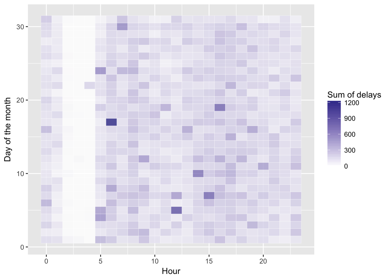
Other than a reliable band of calm very early in the morning, no obvious patterns here.
We need to identify any days that are a Friday the 13th. We also might want to compare weekends, regular Fridays, other weekdays, and Friday the 13ths, so we add a type column that provides these values. Here we use the case_when function:
delays <- delays %>%
    dplyr::mutate(type = case_when( # Partition into Friday the 13ths, Fridays, weekends, and weekdays
      lubridate::wday(.$date) %in% c(1, 7) ~ "weekend",
      lubridate::wday(.$date) %in% c(6) &
        lubridate::day(.$date) == 13 ~ "Friday 13th",
      lubridate::wday(.$date) %in% c(6) ~ "Friday",
      TRUE ~ "weekday" # Everything else is a weekday
  )) %>%
  dplyr::mutate(type = factor(type)) %>%
  dplyr::group_by(type)
delays
## # A tibble: 69,043 x 3
## # Groups:   type [4]
##                   date delay    type
##                 <dttm> <dbl>  <fctr>
##  1 2014-01-01 02:06:00     3 weekday
##  2 2014-01-01 02:40:00     0 weekday
##  3 2014-01-01 03:10:00     3 weekday
##  4 2014-01-01 03:20:00     5 weekday
##  5 2014-01-01 03:29:00     0 weekday
##  6 2014-01-01 07:31:00     0 weekday
##  7 2014-01-01 07:32:00     0 weekday
##  8 2014-01-01 07:34:00     0 weekday
##  9 2014-01-01 07:34:00     0 weekday
## 10 2014-01-01 07:53:00     0 weekday
## # ... with 69,033 more rows
With the data organized, we can start with just a simple box plot of the minutes of delay by type.
ggplot2::ggplot(delays, aes(type, delay)) +
  ggplot2::geom_boxplot() +
  ggplot2::labs(x = "Type", y = "Minutes of delay")
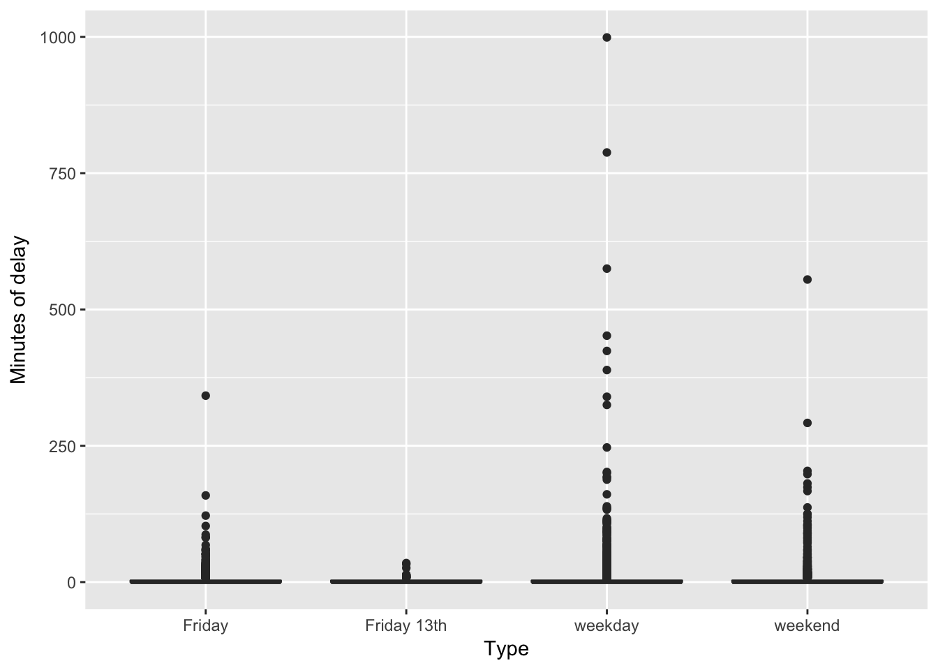
Not very compelling. Basically most delays are short (as in zero minutes long) with many outliers.
How about if we summed up the total minutes in delays for each of the types of days?
delays %>%
  dplyr::summarise(total_delay = sum(delay))
## # A tibble: 4 x 2
##          type total_delay
##        <fctr>       <dbl>
## 1      Friday       18036
## 2 Friday 13th         619
## 3     weekday       78865
## 4     weekend       28194
Clearly the total minutes of delays are much shorter for Friday the 13ths. But, there aren’t very many such days (only 6 in fact). So, this is a dubious analysis.
Let’s take a step back and calculate the average of the total delay across the entire day for each of the types of days. If Friday the 13ths really are unlucky, we would expect to see longer delays, at least relative to a regular Friday.
daily_delays <- delays %>% # Total delays in a day
  dplyr::mutate(year = lubridate::year(date),
                day = lubridate::yday(date)) %>%
  dplyr::group_by(year, day, type) %>%
  dplyr::summarise(total_delay = sum(delay))

mean_daily_delays <- daily_delays %>% # Average delays in each type of day
  dplyr::group_by(type) %>%
  dplyr::summarise(avg_delay = mean(total_delay))
mean_daily_delays
## # A tibble: 4 x 2
##          type avg_delay
##        <fctr>     <dbl>
## 1      Friday 107.35714
## 2 Friday 13th 103.16667
## 3     weekday 113.63833
## 4     weekend  81.01724
ggplot2::ggplot(daily_delays, aes(type, total_delay)) +
  ggplot2::geom_boxplot() +
  ggplot2::labs(x = "Type", y = "Total minutes of delay")
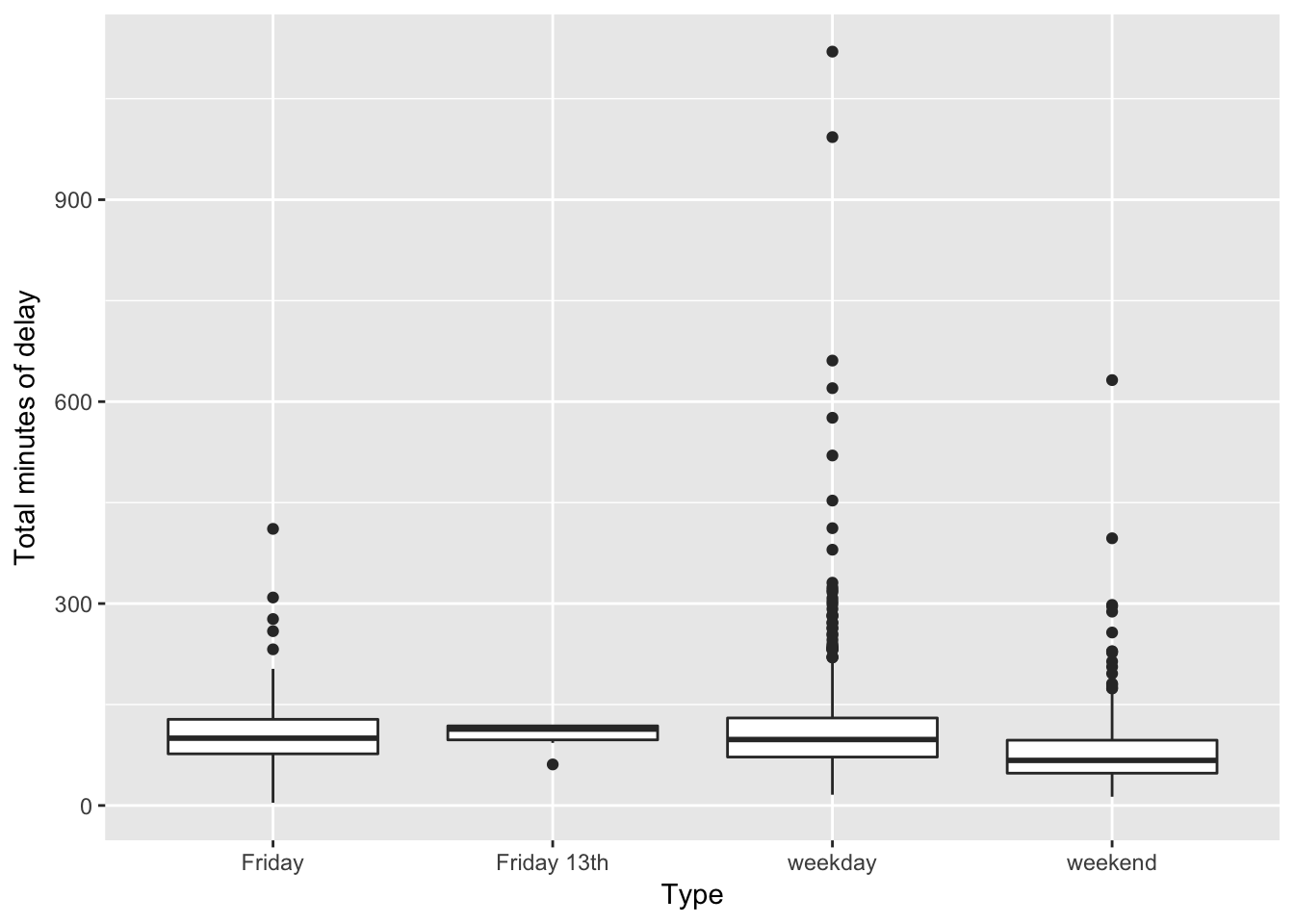
On average, Friday the 13ths have shorter total delays (103 minutes) than either regular Fridays (107 minutes) or other weekdays (114 minutes). Overall, weekend days have far shorter total delays (81 minutes).
If Friday the 13ths are unlucky, they certainly aren’t causing longer TTC delays.
For the statisticians among you that still aren’t convinced, we’ll run a basic linear model to compare Friday the 13ths with regular Fridays. This should control for many unmeasured variables.
model <- lm(total_delay ~ type, data = daily_delays,
            subset = type %in% c("Friday", "Friday 13th"))
summary(model)
##
## Call:
## lm(formula = total_delay ~ type, data = daily_delays, subset = type %in%
##     c("Friday", "Friday 13th"))
##
## Residuals:
##      Min       1Q   Median       3Q      Max
## -103.357  -30.357   -6.857   18.643  303.643
##
## Coefficients:
##                 Estimate Std. Error t value Pr(>|t|)
## (Intercept)      107.357      3.858  27.829   <2e-16 ***
## typeFriday 13th   -4.190     20.775  -0.202     0.84
## ---
## Signif. codes:  0 '***' 0.001 '**' 0.01 '*' 0.05 '.' 0.1 ' ' 1
##
## Residual standard error: 50 on 172 degrees of freedom
## Multiple R-squared:  0.0002365,  Adjusted R-squared:  -0.005576
## F-statistic: 0.04069 on 1 and 172 DF,  p-value: 0.8404
Definitely no statistical support for the idea that Friday the 13ths cause longer TTC delays.
How about time series tests, like anomaly detections? Seems like we’d just be getting carried away. Part of the art of statistics is knowing when to quit.
In conclusion, then, after likely far too much analysis, we find no evidence that Friday the 13ths cause an increase in the length of TTC delays. This certainly suggests that Friday the 13ths are not unlucky in any meaningful way, at least for TTC riders.
Glad we could put this superstition to rest!