I really enjoyed this Strong Song episode on one of my favourite songs: Paranoid Android 🎵
I really enjoyed this Strong Song episode on one of my favourite songs: Paranoid Android 🎵
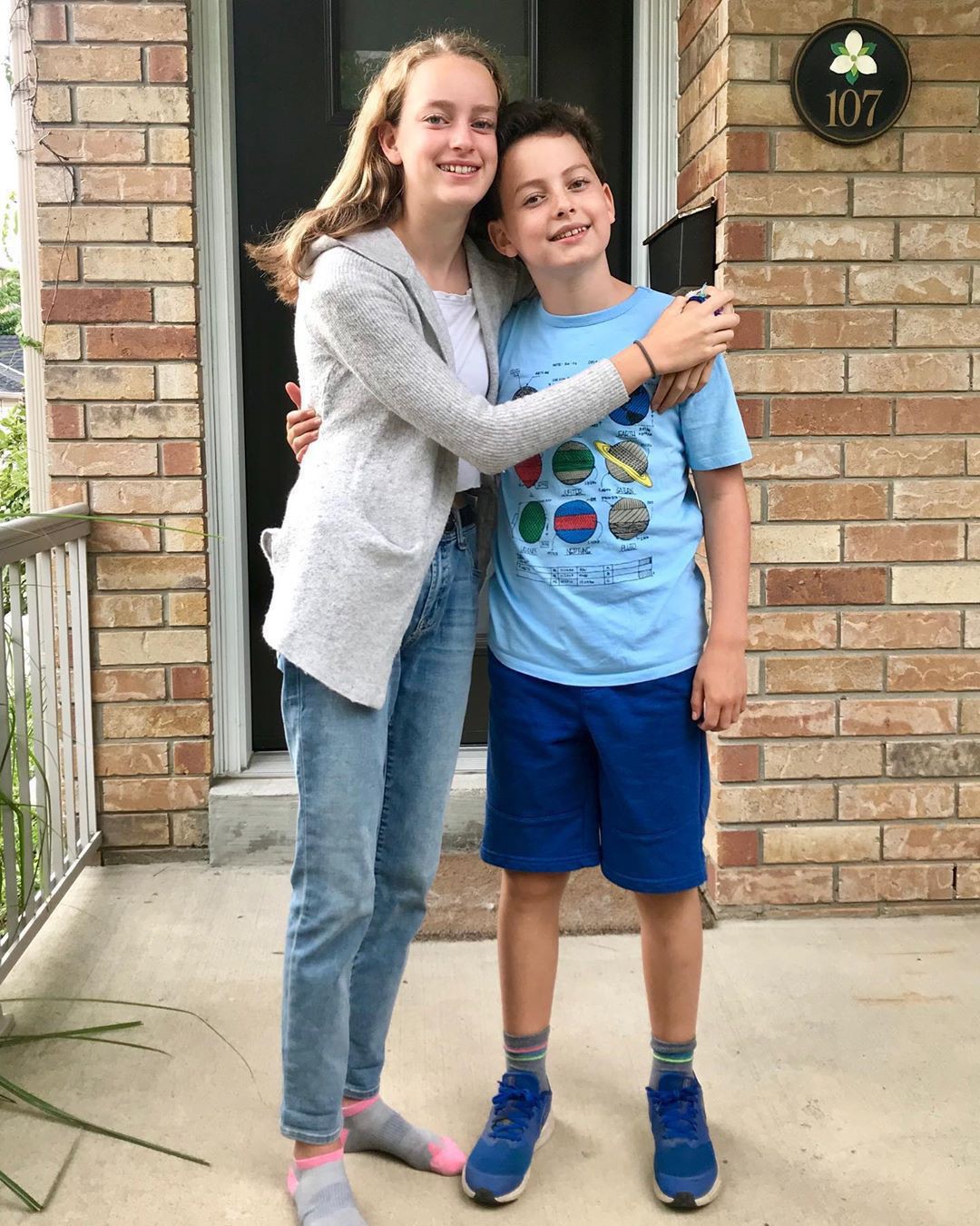
Grades 9 and 6
The Fall by Neal Stephenson is well worth a read. The concepts about consciousness, computer simulations, and death were fascinating, along with the usual hyper detail from Stephenson. Definitely a marathon of a read with multiple, overlapping stories within the book 📚
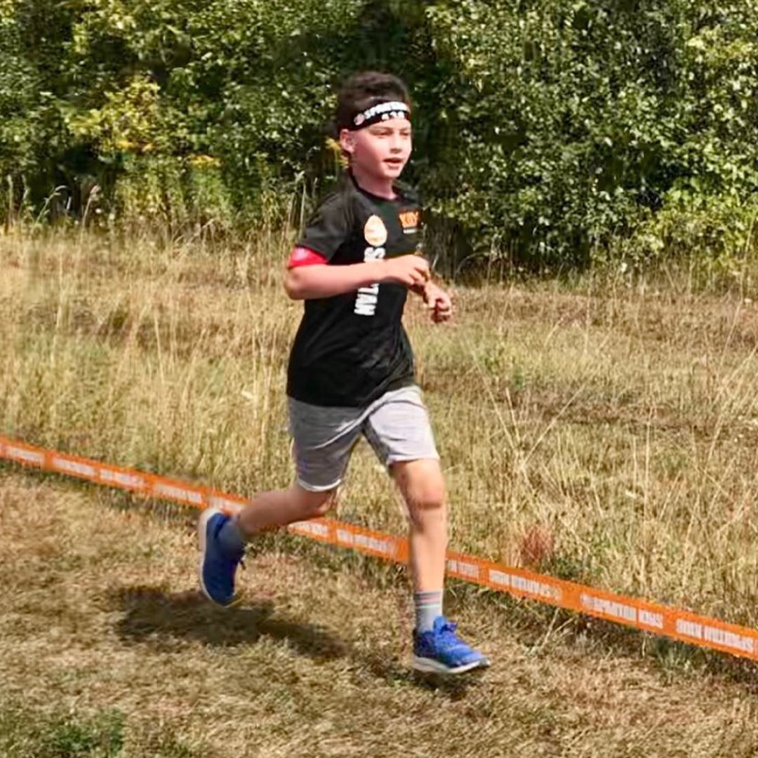
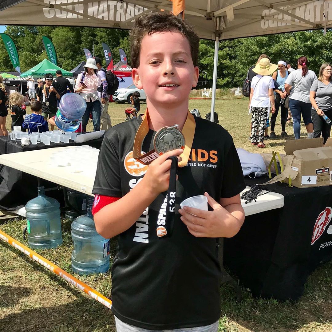
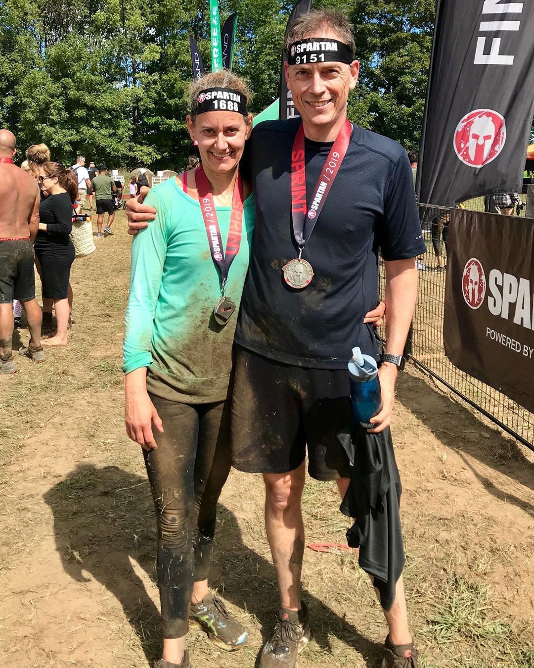
Owen conquered his first #spartantoronto race

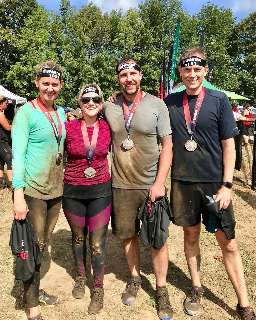
Very fun and very muddy #spartantoronto race

We often think of fungi or other microbes as not particularly intelligent. This study goes to show that across these networks, one of the reasons they can be so successful is that they can make what seem to be fairly sophisticated decisions about where to allocate resources to optimize the return they get.
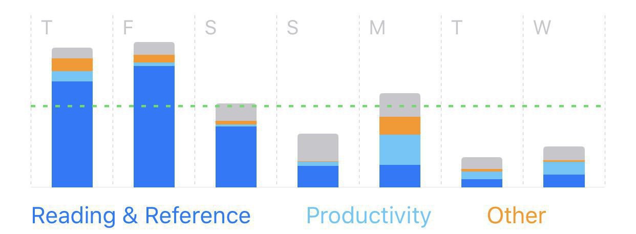
My vacation transition in Screen Time:
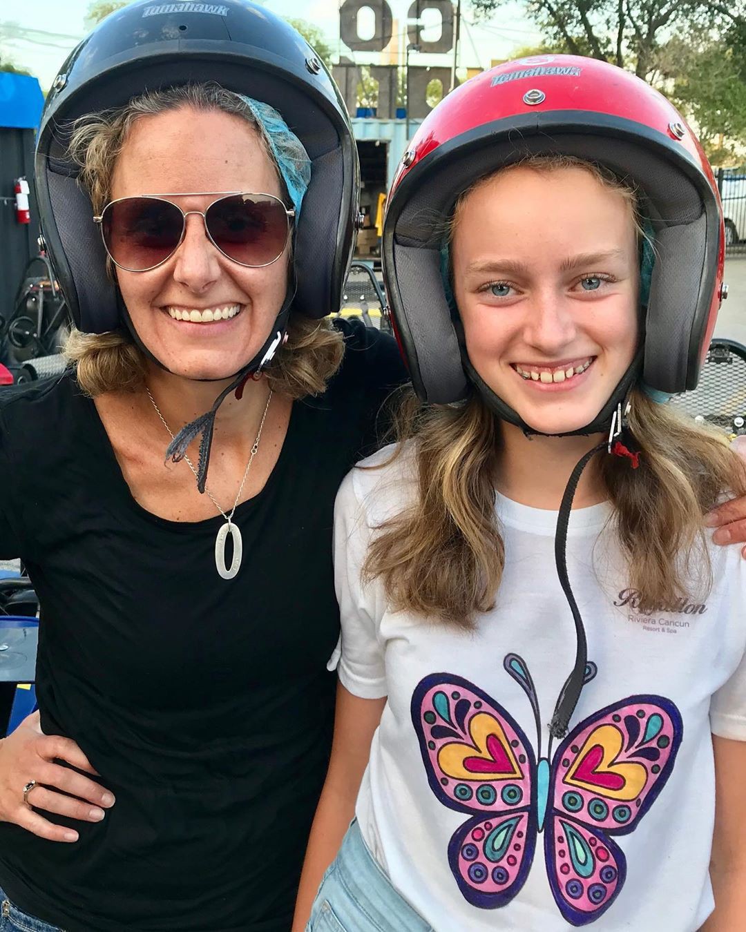
Go Karts!
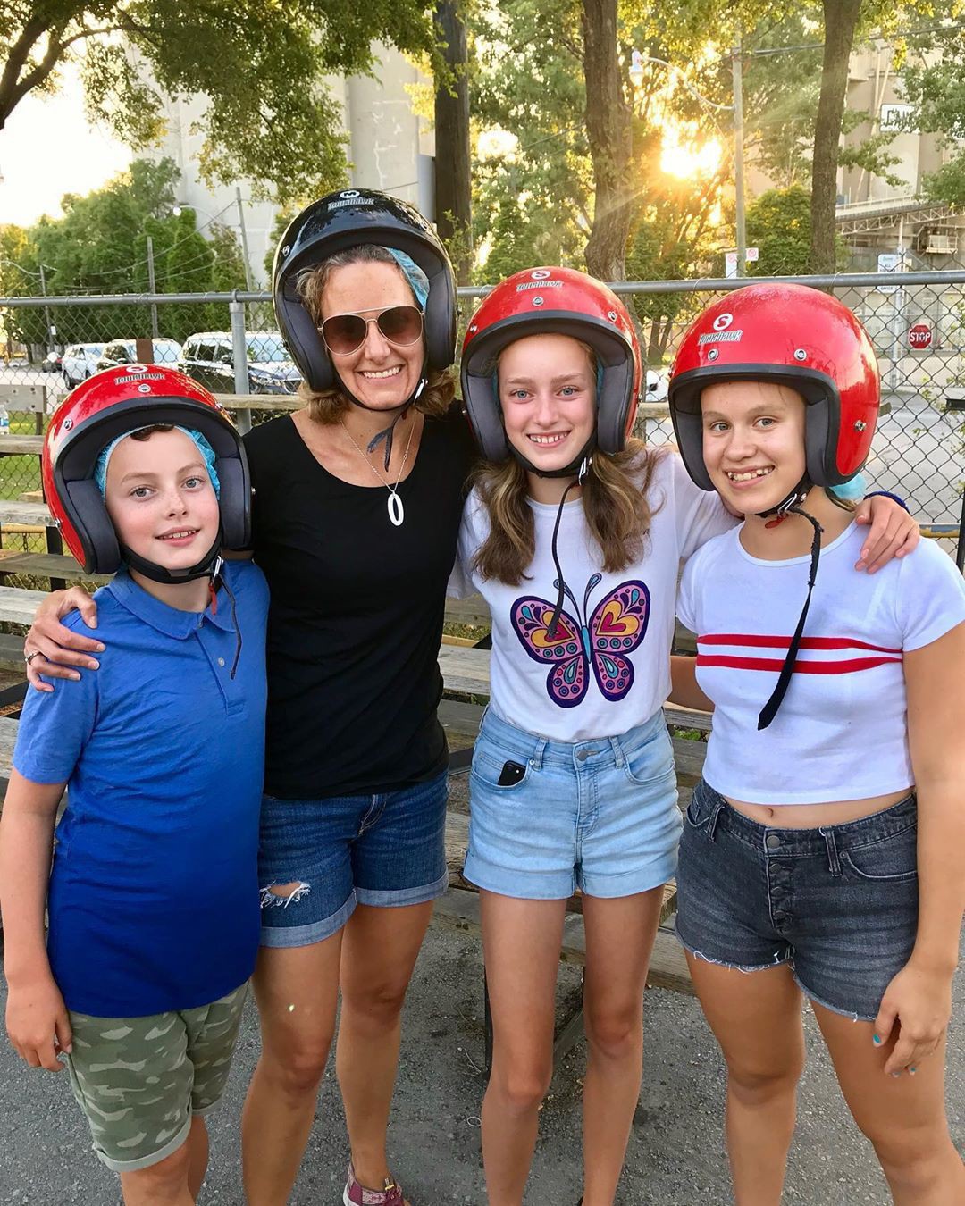
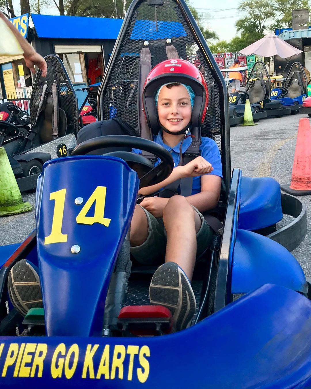
Waiting for the thunderstorms to pass ⛈
Admittedly I didn’t have high expectations, but the First Formic War series from Orson Scott Card and Aaron Johnston is pretty good. Not as sophisticated as the original Ender’s War series, though well worth a vacation read 📚
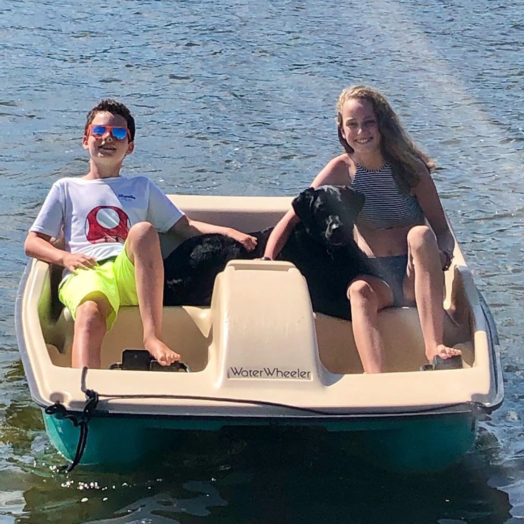
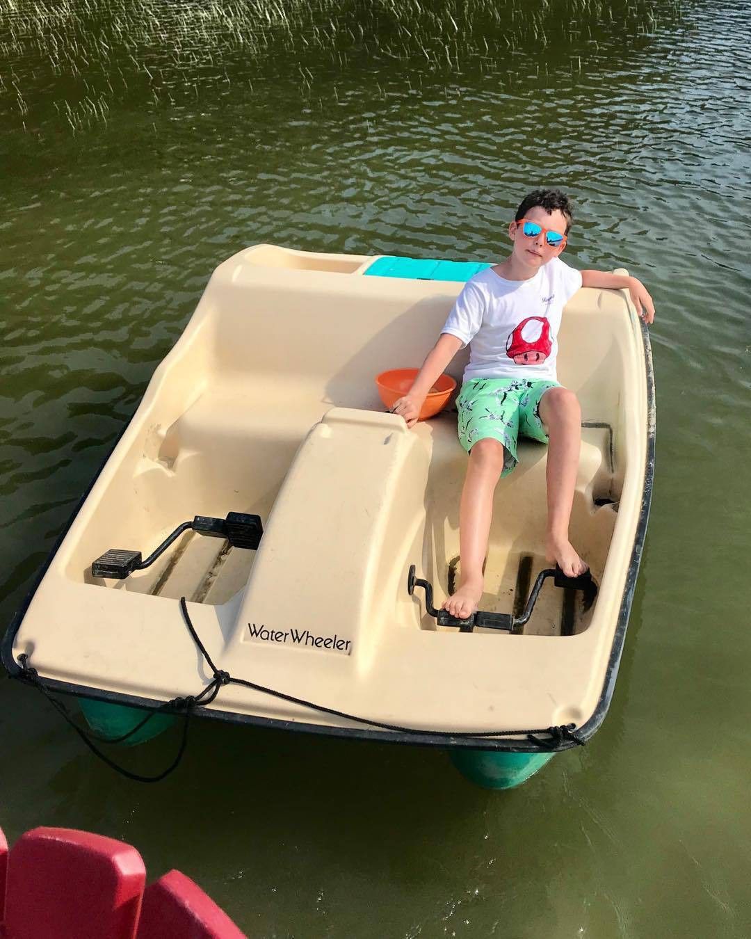
Paddle boat for three
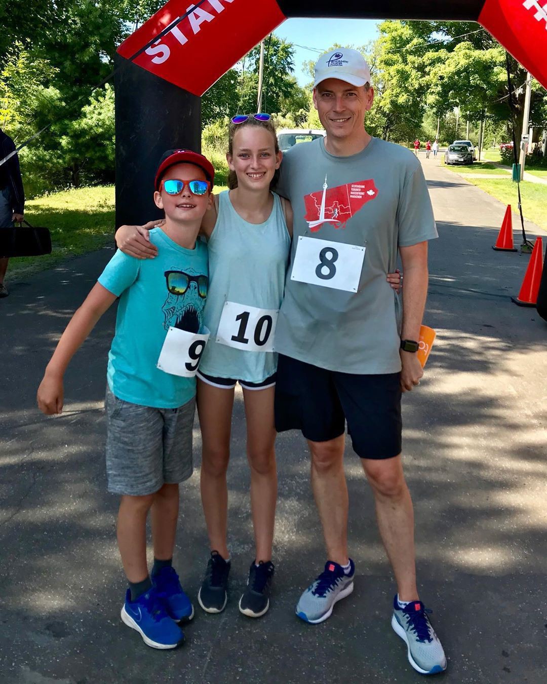
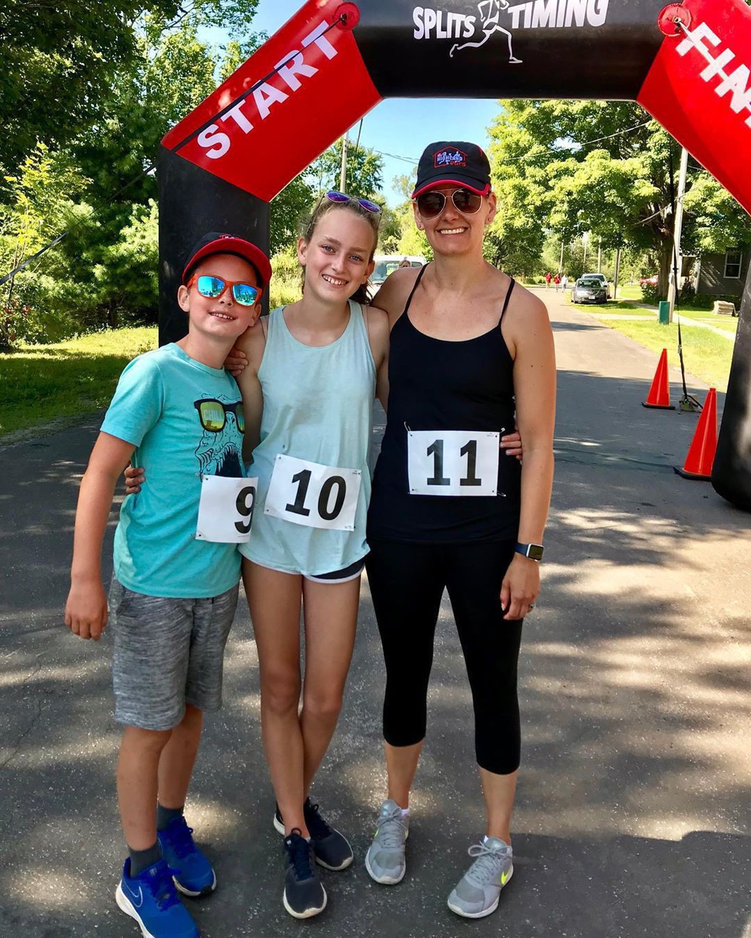
Another great @highlandyardrace, in support of Places for People. An extra thanks to @boshkungbrewing for the refreshing, post-race beer
Chips in the paddle boat
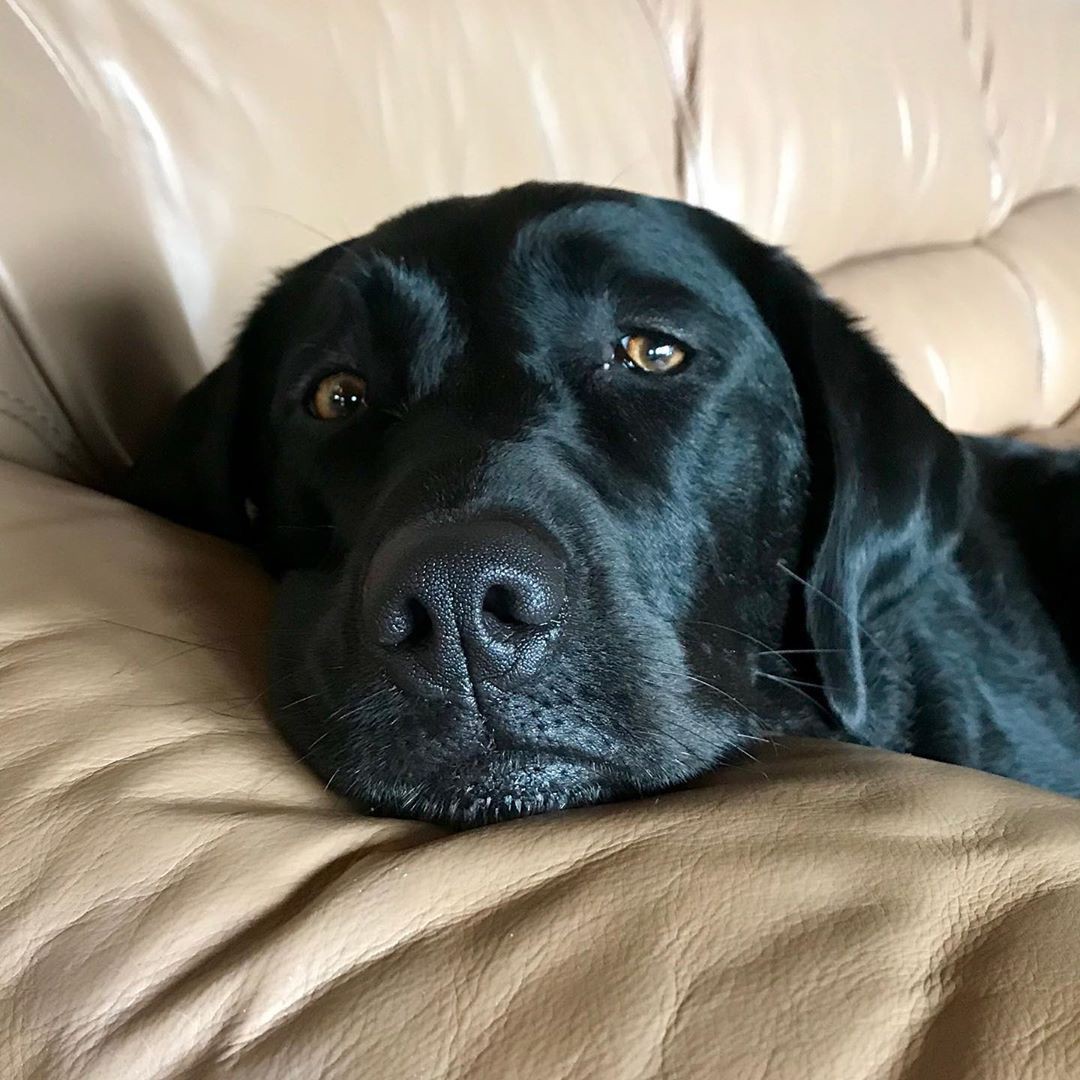
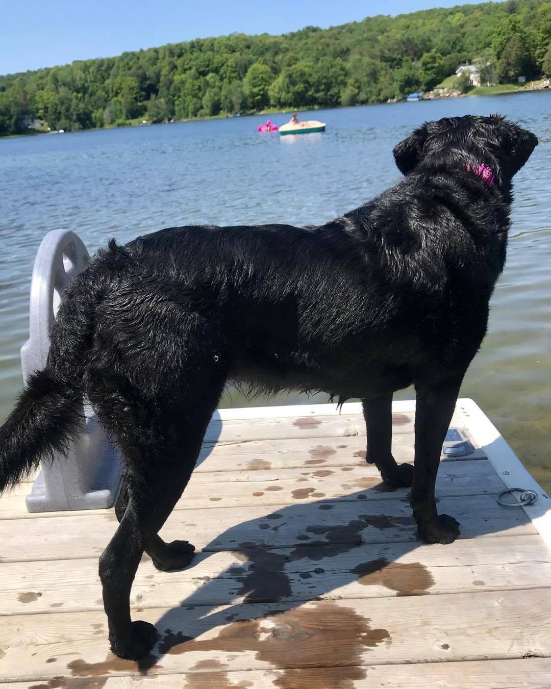
Lucy the lifeguard
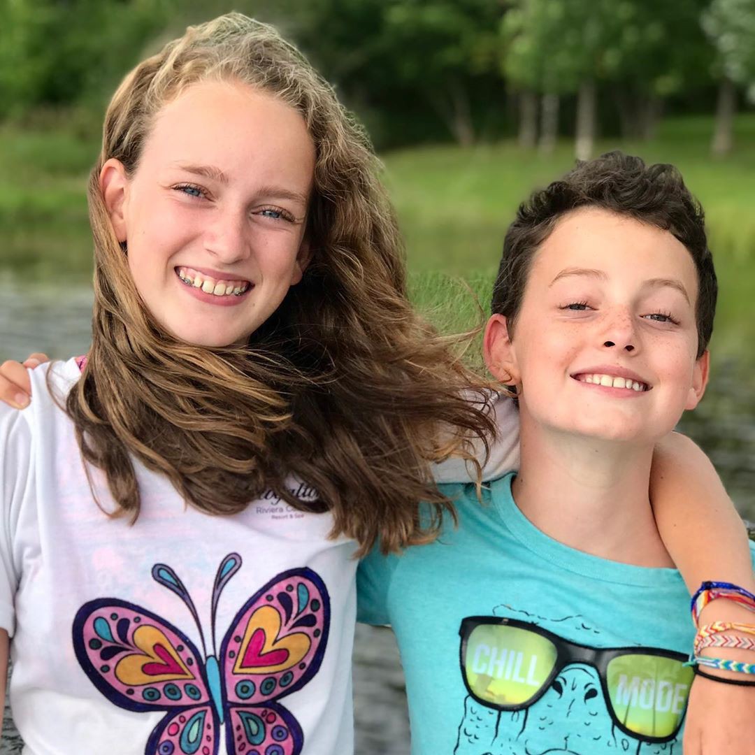
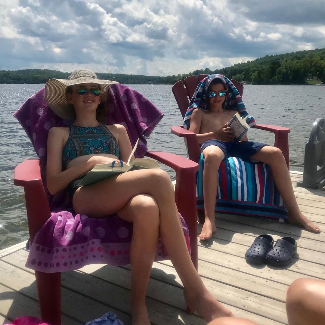
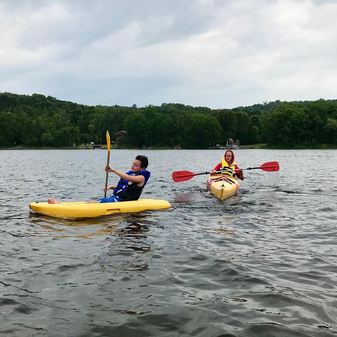
Kids have settled into cottage life
Earth Unaware by Orson Scott Card and Aaron Johnston is a promising start to the prequels for Ender’s Game. Some similarities with the Expanse series, in terms of the asteroid miners, that gives some nice realism to the story and good foreshadowing of the later books 📚
Why We Sleep by Matthew Walker is fascinating and concerning. I knew sleep was important, but not that it is so essential to health, memory, and learning. I’ve been falling short of my 8 hour target for a while now and am definitely motivated to reprioritize sleep again 📚
Conscious by Annaka Harris is a fascinating overview of the science of this mysterious process. Her description of panpsychism was particularly intriguing 📚
The Good Place is a fun, clever show, once you get past the first few episodes 📺