A good read on the mathematics of scaling in urban patterns. I had looked into using the Bettencourt paper (cited in this article) for making allocation decisions. The trick is moving from the general patterns observed in urban scaling to specific recommendations for where to invest in new infrastructure. This is particularly challenging in the absence of good, detailed data on the current infrastructure stock. We’ve made good progress on gathering some of this data, and it might be worth revisiting this scaling relationship.
I’m certain that paying attention to where my food comes from is important. Food production influences my health, has environmental consequences, and affects both urban and rural design. Ideally, I would develop relationships with local farmers, carefully choose organic produce, and always consider broad environmental impacts. Except, I like to spend time with my young family, try to get some exercise, and have more than enough commitments through work to actually spend this much effort on food choices. So, I’ve outsourced this process to the excellent Mama Earth Organics.
Every week a basket of fresh organic and/or local fruit and vegetables arrives on our doorstep. Part of the fun of this service is that different items arrive each week, which diversifies our weekly food routine. But, we always know what’s coming several days in advance, so we can plan our meals well ahead of time. After over a year of service, we’ve only had a single complaint about quality and this was handled very quickly by Mama Earth with a full refund plus credit.
We’ve found the small basket is sufficient for two adults and a picky four-year old. We’ve also added in some fresh bread from St. John’s Bakery, which has been consistently delicious and lasts through most of the week.
When it comes to the Canadian economy, Obama may as well be PM
An important discussion of how US energy policy is driving Canadian policy.
Commercial air travel, like many other industries, is lubricated by cheap oil. Mr. Rubin, the former chief economist of CIBC World Markets, has now bet his career on a single idea – that the cheap oil era is dead and globalization is about to wither along with it. But the most fascinating part of his thesis has nothing to do with geology or Hubbert’s peak oil theory. It’s about the reindustrialization of North America. Those unemployed airline workers could be looking for work – and finding it – in the revitalized factories of Southern Ontario.
… in Saskatoon today, Bay Street investors and a group of chiefs from Saskatchewan and Alberta will formally announce the unlikeliest of marriages, one that will make them the most influential farmers in all of Canada, with a super-sized one-million-acre operation that could rival the largest corporate farms in the world.
Under the plan, 17 native bands will lease their land at market value to a new entity called One Earth Farms Corporation, which will focus on sustainable, environmentally responsible land use, hire and train aboriginal workers, and provide first nations an equity stake in the company.
This is an interesting initiative and worth tracking – not because of the massive size of the project. Rather, the partnership between bands and investors is novel.
Our minister of science continues to argue that his unwillingness to endorse the theory of evolution is not relevant to science policy. As quoted by the Globe and Mail:
My view isn’t important. My personal beliefs are not important.
I find this amazing. How can the minister of science’s views on the fundamental unifying theory of biology not be important?
I don’t expect him to understand the details of evolutionary theory or to have all of his personal beliefs vetted and religious views muted. However, I do expect him – as minister – to champion and support Canadian science, especially basic research. When our minister refuses to acknowledge the fundamental discoveries of science, our reputation is diminished.
There is also a legitimate – though rather exaggerated – concern that the minister’s views on the truth can influence policy and funding decisions. The funding councils are more than sufficiently independent to prevent any undue ministerial influence here. The real problem is an apparent distrust or lack of interest in basic research from the federal government.
If only there were some institution that had a reputation for journalistic integrity that had a staff of trained editors and a growing audience arriving at its web site every day seeking quality information. If only… Of course, we have thousands of these institutions. They’re called newspapers.
Canada says it has legal obligation to prevent Abdelrazik from travelling: Other terrorism suspects have returne.. theglobeandmail.com/servlet…
This has to stop. Abdelrazik is a Canadian citizen and should be allowed to return. I don’t understand what the Canadian Government is trying to accomplish here.
His main point is certainly right: we can’t have the many benefits of energy without consequence and the National Geographic neglected to show these benefits. However, I do think that Canadians need to be aware of the trade-offs we are making and mitigate – to the extent possible – threats to our environment. For most of us, energy just appears when we flip a switch or drive to the gas station.
I think the tar sands are an important Canadian resource and with careful stewardship their benefits could far exceed their costs. However, my sense is that current policies are not focussed on stewardship and we risk squandering the opportunities provided by the tar sands.
But here’s a surprise for Stephen Harper. We’re calling your bluff. This time we’re telling Ottawa: not so fast. Lots of Canadians are prepared to risk prosecution and defy the ban on funding Abdelrazik. Through an explicit civil disobedience project called Operation Fly Home, spearheaded by Mary Foster in Montreal, a first group of 115 Canadians have so far donated small sums to buy his air ticket home. All of us are making our names and addresses public, so the Mounties won’t have trouble finding us. Our crime? Paying $20 dollars or so to bring home a stranded fellow Canadian whose only crime is his name and religion.
“Operation Fly Home” is a great initiative in response to this bizarre government behaviour.
Fatal Distraction: Forgetting a Child in the Backseat of a Car Is a Horrifying Mistake. Is It a Crime? Gene Weingarten Reports.
“Death by hyperthermia” is the official designation. When it happens to young children, the facts are often the same: An otherwise loving and attentive parent one day gets busy, or distracted, or upset, or confused by a change in his or her daily routine, and just… forgets a child is in the car. It happens that way somewhere in the United States 15 to 25 times a year, parceled out through the spring, summer and early fall. The season is almost upon us.
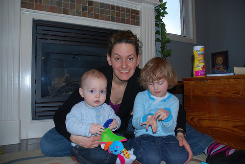
A rare shot of Kelly with both kids. If only we could get Owen and Emma to look at the camera simultaneously.
Sure, science isn’t that exciting. It tends to offer up steady, incremental bits of knowledge rather than miraculous cures, and there remain a lot of unknowns. But these voids need not be filled with fantasy and snake oil.
And, yes, Big Pharma and big business have had their scandals and excesses, but these have been exposed and denounced by the so-called establishment, and they do not negate the good.
Over time, there has emerged from this “vast conspiracy” pretty good health care.
Daring Fireball: Observations, Complaints, Quibbles, and Suggestions Regarding the Safari 4 Public Beta Released One Week Ago, Roughly in Order of Importance
A great example of why I read Daring Fireball: strongly held and insightful opinions, backed by tremendous research and detail.
My plea to all Internet commentators is to at least step up to a certain level of wit and discourse when you publicly disagree, and to challenge the source of your own anger before you spew it at someone else.
But I don’t think that is going too happen any time soon. People out there are having way too much fun to stop the hate.